Centauri Dreams
Imagining and Planning Interstellar Exploration
A Better Look at 3I/ATLAS
Just a short note, prompted by the release of new imagery of the intersellar object 3I/ATLAS by the Gemini North telescope in Hawaii. It’s startling how quickly we’ve moved from the first pinpoint images of this comet to what we see below, which draws on Gemini North’s Multi-Object Spectrograph to show us the tight (thus far) coma of the object, the gas and dust cloud enshrouding its nucleus. Changes here as the comet nears perihelion will teach us much about the object’s composition and size. Some early estimates have the cometary nucleus as large as 20 kilometers, considerably larger than both ‘Oumuamua and 2I/Borisov, the first two such objects detected. This is a figure that will doubtless be adjusted with continued observation.
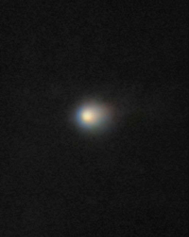
Image: Using the Gemini North telescope, astronomers have captured 3I/ATLAS as it makes its temporary passage through our cosmic neighborhood. These observations will help scientists study the characteristics of this rare object’s origin, orbit, and composition. Credit: NSF NOIRLab.
3I/ATLAS also shows a more eccentric orbit than its predecessors. Remember that an eccentricity of 0 means an orbit that is completely circular, while as we move from 0 to 1, the orbit becomes drawn out, to the point where an orbit with eccentricity values of 1 or above doesn’t return to the Sun, but continues into interstellar space. The new comet’s orbital eccentricity is 6.2, considerably higher than ‘Oumuamua (1.2) and Borisov (3.6). Perihelion will come at the end of October at a distance of 210 million kilometers, which will place the object just inside the orbit of Mars. Amateur astronomers with a good telescope may just be able to get a glimpse of it late in 2025.

A New Horizons First for Interstellar Navigation
If you’re headed for another planet, celestial markers can keep your spacecraft properly oriented. Mariner 4 used Canopus, a bright star in the constellation Carina, as an attitude reference, its star tracker camera locking onto the star after its Sun sensor had locked onto the Sun. This was the first time a star had been used to provide second axis stabilization, its brightness (second brightest star in the sky) and its position well off the ecliptic making it an ideal referent.
The stars are, of course, a navigation tool par excellence. Mariners of the sea-faring kind have used celestial navigation for millennia, and I vividly remember a night training flight in upstate New York when my instructor switched off our instrument panel by pulling a fuse and told me to find my way home. I was forcefully reminded how far we’ve come from the days when the night sky truly was a celestial map for travelers. Fortunately, a few bright cities along the way made dead reckoning an easy way to get home that night. But I told myself I would learn to do better at stellar navigation. I can still hear my exasperated instructor as he pointed out one celestial marker: “For God’s sake, see that bright star? Park it over your left wingtip!”
Celestial navigation of various kinds can be done aboard a spacecraft, and the use of pulsars will help future deep space probes navigate autonomously. Until then, our methods rely heavily on ground-based installations. Delta-Differential One-Way Ranging (Delta-DOR or ∆DOR) can measure the angular location of a target spacecraft relative to a reference direction, the latter being determined by radio waves from a source like a quasar, whose angular position is well known. Only the downlink signal from the spacecraft is used in a precision technique that has been employed successfully on such missions as China’s Chang’e, ESA’s Rosetta and NASA’s Mars Reconnaissance Orbiter.
The Deep Space Network and Delta-DOR can perform marvels in terms of the directional location of a spacecraft. But we’ve also just had a first in terms of autonomous navigation through the work of the New Horizons team. Without using radio tracking from Earth, the spacecraft has determined its distance and direction by examining images of star fields and the observed parallax effects. Wonderfully, the two stars that the team chose for this calculation were Wolf 359 and Proxima Centauri, two nearby red dwarfs of considerable interest.
The images in question were captured by New Horizons’ Long Range Reconnaissance Imager (LORRI) and studied in relation to background stars. These twp stars are almost 90 degrees apart in the sky, allowing team scientists to flag New Horizons’ location. The LORRI instrument offers limited angular resolution and is here being used well outside the parameters for which it was designed, but even so, this first demonstration of autonomous navigation didn’t do badly, finding a distance close to the actual distance of the spacecraft when the images were taken, and a direction on the sky accurate to a patch about the size of the full Moon as seen from Earth. This is the largest parallax baseline ever taken, extending for over four billion miles. Higher resolution imagers, as reported in this JHU/APL report, should be able to do much better.
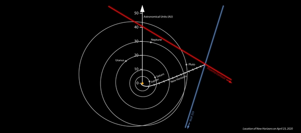
Image: Location of NASA’s New Horizons spacecraft on April 23, 2020, derived from the spacecraft’s own images of the Proxima Centauri and Wolf 359 star fields. The positions of Proxima Centauri and Wolf 359 are strongly displaced compared to distant stars from where they are seen on Earth. The position of Proxima Centauri seen from New Horizons means the spacecraft must be somewhere on the red line, while the observed position of Wolf 359 means that the spacecraft must be somewhere on the blue line – putting New Horizons approximately where the two lines appear to “intersect” (in the real three dimensions involved, the lines don’t actually intersect, but do pass close to each other). The white line marks the accurate Deep Space Network-tracked trajectory of New Horizons since its launch in 2006. The lines on the New Horizons trajectory denote years since launch. The orbits of Jupiter, Saturn, Uranus, Neptune and Pluto are shown. Distances are from the center of the solar system in astronomical units, where 1 AU is the average distance between the Sun and Earth. Credit: NASA/Johns Hopkins APL/SwRI/Matthew Wallace.
Brian May, known for his guitar skills with the band Queen as well as his knowledge of astrophysics, helped to produce the images below that show the comparison between these stars as seen from Earth and from New Horizons. A co-author of the paper on this work, May adds:
“It could be argued that in astro-stereoscopy — 3D images of astronomical objects – NASA’s New Horizons team already leads the field, having delivered astounding stereoscopic images of both Pluto and the remote Kuiper Belt object Arrokoth. But the latest New Horizons stereoscopic experiment breaks all records. These photographs of Proxima Centauri and Wolf 359 – stars that are well-known to amateur astronomers and science fiction aficionados alike — employ the largest distance between viewpoints ever achieved in 180 years of stereoscopy!”
Here are two animations showing the parallax involving each star, with Proxima Centauri being the first image. Note how the star ‘jumps’ against background stars as the view from Earth is replaced by the view from New Horizons.
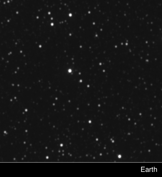
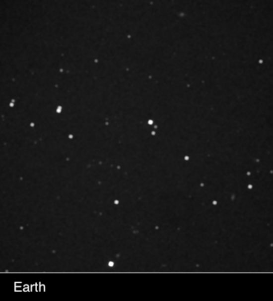
Image: In 2020, the New Horizons science team obtained images of the star fields around the nearby stars Proxima Centauri (top) and Wolf 359 (bottom) simultaneously from New Horizons and Earth. More recent and sophisticated analyses of the exact positions of the two stars in these images allowed the team to deduce New Horizons’ three-dimensional position relative to nearby stars – accomplishing the first use of stars imaged directly from a spacecraft to provide its navigational fix, and the first demonstration of interstellar navigation by any spacecraft on an interstellar trajectory. Credit: JHU/APL.
This result from New Horizons marks the first time that optical stellar astrometry has been applied to the navigation of a spacecraft, but it’s clear that our hitherto Earth-based methods of navigation in space will have to give way to on-board methods as we venture still farther out of the Solar System. Thus far the use of X-ray pulsars has been demonstrated only in Earth orbit, but it will surely be among the techniques employed. These rudimentary observations are likewise proof-of-concept whose accuracy will need dramatic improvement.
The paper notes the next steps in using parallactic measurements for autonomous navigation:
Considerably better performance should be possible using the cameras presently deployed on other interplanetary spacecraft, or contemplated for future missions. Telescopes with apertures plausibly larger than LORRI’s, with diffraction-limited optics, delivering images to Nyquist-sampled detectors [a highly accurate digital signal processing method], mounted on platforms with matching finepointing control, should be able to provide astrometry with few milli-arcsecond accuracy. Extrapolating from LORRI, position vectors with accuracy of 0.01 au should be possible in the near future.
The paper on this work is Lauer et al., “A Demonstration of Interstellar Navigation Using New Horizons,” accepted at The Astronomical Journal and available as a preprint.
3I/ATLAS: Observing and Modeling an Interstellar Newcomer
Let’s run through what we know about 3I/ATLAS, now accepted as the third interstellar object to be identified moving through the Solar System. It seems obvious not only that our increasingly powerful telescopes will continue to find these interlopers, but that they are out there in vast numbers. A calculation in 2018 by John Do, Michael Tucker and John Tonry (citation below) offers a number high enough to make these the most common macroscopic objects in the galaxy. But that may well depend on how they originate, a question of lively interest and one that continues to produce papers.
Let me draw on a just released preprint from Matthew Hopkins (University of Oxford) and colleagues that runs through the formation options. Pointing out that interstellar object (ISO) studies represent an entirely new field, they note that theoretical thinking about such things trended toward comets as the main source, an idea immediately confronted by ‘Oumuamua, which appeared inert even as it drew closer to the inner system and even appeared to accelerate as it departed. The controversy over its origin made 2I/Borisov a relatively tame object, it being clearly a comet. 3I/ATLAS looks a lot more like 2I/Borisov than ‘Oumuamua, though it’s larger than either.
Protoplanetary disks are a possible source of interstellar debris, but so for that matter are the Oort-like clouds that likely surround most main sequence stars, and that would largely be released when their hosts complete their evolution. ‘Oumuamua has been analyzed as a fragment of a small, outer-system world around another star, or even as a ‘hydrogen iceberg,’ and I see there is one paper suggesting that ISOs may be a part of galactic renewal, contributing their materials into protoplanetary disks and nascent planets.
The Hopkins paper underlines the ubiquity of such objects:
A standard picture has emerged, in which planetesimals formed within a protoplanetary disk are scattered by interactions with migrating planets or via stellar flybys, early in the history of a system (Fitzsimmons et al. 2023). The number density inferred from observations of the first two ISOs, in addition to studies of scattering in our own Solar System, suggest that such events are common, with ≳ 90% of planetesimals joining the ISO population (Jewitt & Seligman 2023). Such objects spread around the Milky Way’s disk in braided streams (Forbes et al. 2024), a small fraction of which intersect our Solar System. The observed ISO population is thus truly galactic, rather than being associated with local stars and stellar populations.
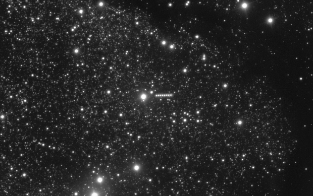
Image: ESO’s Very Large Telescope (VLT) has obtained new images of 3I/ATLAS, an interstellar object discovered in recent weeks. Identified as a comet, 3I/ATLAS is only the third visitor from outside the Solar System ever found, after 1I/ʻOumuamua and 2I/Borisov. Its highly eccentric hyperbolic orbit, unlike that of objects in the Solar System, gave away its interstellar origin. In this image, several VLT observations have been overlaid, showing the comet as a series of dots that move towards the right of the image over the course of about 13 minutes on the night of 3 July 2025. The data were obtained with the FORS2 instrument, and are available in the ESO archive. Credit: European Southern Observatory.
I’m struck anew by how much our view of our Solar System’s place in the cosmos has changed. The size and density of the Kuiper Belt only swam into focus when the first KBO was discovered in 1992, although the belt had been hypothesized by Kenneth Edgeworth in the 1930s and Gerald Kuiper in 1951. The vast Oort Cloud of comets that envelops our entire system was posited by Jan Hendrik Oort in 1950. Now we’re looking at populations of objects at minute sub-planetary scale existing between the stars in unfathomable numbers.
Hopkins and team point out that the Rubin Observatory Legacy Survey of Space and Time (LSST) will dramatically increase the number of confirmed ISOs. So then, what do we have on 3I/ATLAS? The early work on the object identifies it as a comet with a compact coma, a cloud of gas and dust surrounding the nucleus. It’s also bigger than its two predecessors, perhaps as large as 10 kilometers, as opposed to ‘Oumuamua and Borisov’s roughly 0.1 kilometers, although a more precise number will emerge as we learn more about its composition and albedo. It enters the Solar System at a higher speed than the latter ISOs, but one well within the distribution model used in this paper.
Interestingly, the object shows high vertical motion out of the plane of the galaxy, ruling out the idea that it comes from the same star as ‘Oumuamua or Borisov. That velocity points to an origin in the Milky Way’s thick disk – stars above and below the disk within which the Solar System resides. It is the first object to be identified as such. Says Hopkins:
“All non-interstellar comets such as Halley’s comet formed with our solar system, so are up to 4.5 billion years old. But interstellar visitors have the potential to be far older, and of those known about so far our statistical method suggests that 3I/ATLAS is very likely to be the oldest comet we have ever seen.”
The team’s model (based on Gaia data, disk chemistry and galactic dynamics) was developed during Hopkins’ doctoral research. It emerges as the first real-time application of predictive modelling to an interstellar comet. It likewise predicts that 3I/ATLAS will have a high water content. We’ll be able to check on that as observations continue. Co-author Michele Bannister, of the University of Canterbury in New Zealand, points out that 3I/ATLAS is already showing activity as it warms during its approach to the Sun. The gases the comet produces as it moves toward perihelion at 1.36 AU in October will tell us more.
The paper is Hopkins et al., “From a Different Star: 3I/ATLAS in the context of the ̄Otautahi–Oxford interstellar object population model,” submitted to Astrophysical Journal Letters and available as a preprint. The paper on the density of the interstellar object population is Do, Tucker & Tonry, “Interstellar Interlopers: Number Density and Origin of ‘Oumuamua-like Objects,” Astrophysical Journal Letters Vol. 855 (6 March 2018), L10. Full text. Also be aware of a new paper by Avi Loeb at Harvard that I haven’t yet had time to review. It’s “Comment on “Discovery and Preliminary Characterization of a Third Interstellar Object: 3I/ATLAS” (preprint).
New Model to Prioritize the Search for Exoplanet Life
Our recent focus on habitability addresses a significant problem. In order for astrobiologists to home in on the best targets for current and future telescopes, we need to be able to prioritize them in terms of the likelihood for life. I’ve often commented on how lazily the word ‘habitable’ is used in the popular press, but it’s likewise striking that its usage varies widely in the scientific literature. Alex Tolley today looks at a new paper offering a quantitative way to assess these matters, but the issues are thorny indeed. We lack, for instance, an accepted definition of life itself, and when discussing what can emerge on distant worlds, we sometimes choose different sets of variables. How closely do our assumptions track our own terrestrial model, and when may this not be applicable? Alex goes through the possibilities and offers some of his own as the hunt for an acceptable methodology continues.
by Alex Tolley
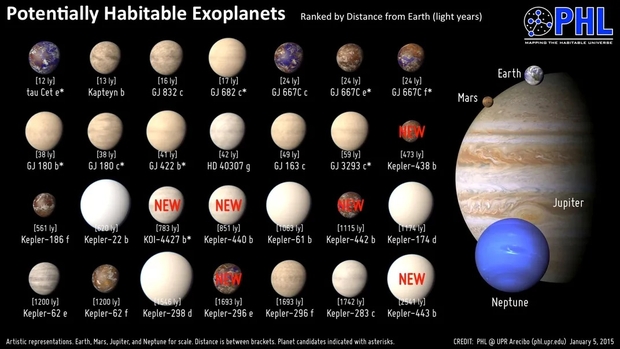
Artist illustrations of explanets in the habitable zone as of 2015. None appear to be illustrated as possible hanbitable worlds. This has changed in the last decade. Credit: PHL @ UPR Arecibo (phl.upr.edu) January 5, 2015 Source [1]
We now know that the galaxy is full of exoplanets, and many systems have rocky planets in their habitable zones (HZ). So how should we prioritize our searches to maximize our resources to confirm extraterrestrial life?
A new paper by Dániel Apai and colleagues of the Quantitative Habitability Science Working Group, a group within the Nexus for Exoplanet System Science (NExSS) initiative, looks at the problems hindering our quest to prioritize searches of the many possible life-bearing worlds discovered to date and continuing to be discovered with new telescope instruments.
The authors state that the problem we face in the search for life is:
“A critical step is the identification and characterization of potential habitats, both to guide the search and to interpret its results. However, a well-accepted, self-consistent, flexible, and quantitative terminology and method of assessment of habitability are lacking.”
The authors expend considerable space and effort itemizing the problems that have accrued: Astrobiologists and institutions have never defined “habitable” and “habitability” rigorously, even confounding “habitable” with “Habitable Zone” (HZ), and using “habitable” and “inhabited” almost interchangeably. They argue that this creates problems for astrobiologists when trying to plan how to develop strategies when determining which exoplanets are worth investigating and how. Therefore, defining terminology is important to avoid confusion. As the authors point out, researchers often assume that planets in the HZ should be habitable and those outside its boundaries uninhabitable, even though both assertions are untrue.
[I am not clear that the first assertion is claimed without caveats, for example, the planet must be rocky and not a gaseous world, such as a mini-Neptune.]
As our knowledge of exoplanets is data poor, it may not be possible to define whether a planet is habitable based on the available information, which leads to the imprecision of the term “habitable”. In addition, not only has “habitable” not been well-defined, but neither have the requirements for life been defined, which is more restrictive than the loose requirement for surface liquid water.
Ultimately, the root of the problem that hampers the community’s efforts to converge on a definition for habitability is that habitability depends on the requirements for life, and we do not have a widely agreed-upon definition for life.
The authors accept that a universal definition of life may not be possible, but that we can, however, determine the habitat requirements of particular forms of life.
The authors’ preferred solution is to model habitability with joint probability assessments of planetary conditions with already acquired data, and extended with new data. This retains some flexibility in the use of the term “habitable” in the light of new data.
Figure 1 below illustrates the various qualitative approaches to defining habitability. Adhering to any single definition is not possible for a universal definition. The paper suggests that a better approach is to use quantitative methods that are both rigorous, yet flexible in the light of new data and information.
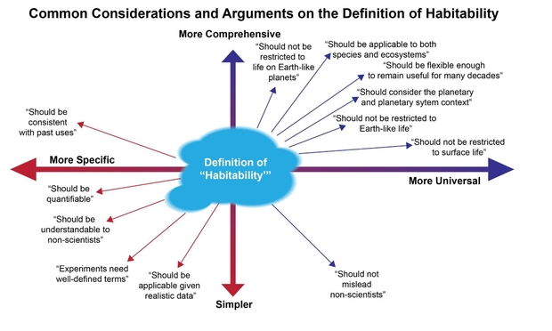
Figure 1. Various approaches to defining “habitable”. Any single definition for “habitability” fails to meet the majority of the requirements.
The equation below illustrates the idea of quantifying the probability of a planet’s habitability as a joint probability of the known criteria:
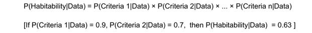
The authors use the joint probability of the planet being habitable. For example, it is in the HZ, is rocky, and has water vapor in the atmosphere. Clearly, under this approach, if water vapour cannot be detected, the probability of habitability declines to zero.
Perhaps of even greater importance, the group also looks at habitability based on whether a planet supports the requirements for known examples of terrestrial life, whose requirements vary considerably. For example, is there sufficient energy to support life? If there is no useful light from the parent star in the habitat, energy must be supplied by geological processes, leading to the likelihood that only anaerobic chemotrophs could live under those conditions, for example, as hypothesized in dark, glacial-covered subsurface oceans..
The authors include more carefully defined terms, including: Earth-like life. Rocky Planet, Earth-Sized Planet, Earth-Like Planet, Habitable Zone, Metabolisms, Viability Model, Suitable Habitat for X, and lastly Habitat Suitability which they defined as:
The measure of the overlap between the necessary environmental conditions for a metabolism and environmental conditions in the habitat.
Because of the probability that life (at least some species of terrestrial life) will inhabit a planet, the authors suggest a framework where the Venn diagram of the probability of a planet being habitable intersects with the probability that the requirements are met for specific species of terrestrial life.
The Quantitative Habitability Framework (QHF) is shown in Figure 2 below.
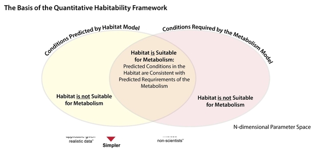
Figure 2. Illustration of the basis of the Framework for Habitability: The comparison of the environmental conditions predicted by the habitat model and the environmental conditions required by the metabolism model.
The probability of the viability of an organism for each variable is a binary value of 0 for non-viability and 1 for viability. For archaea and temperature, this is:
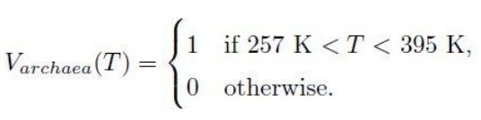
The equation means that the probability of viability of the archaea at temperature T in degrees Kelvin is 1 if the temperature is between 257 K ( -16 °C) and 395 K (122 °C). Otherwise 0 if the temperature is outside the viable range. (Ironically, this is imprecise, as it is for a species of archaean methanogen extremophile, not all archaeans.)
This approach is applied to other variables. If any variable probability is zero, the joint probability of viability becomes 0.
The figure below shows various terrestrial organism types, mostly unicellular, with their known temperature ranges for survival. The model therefore allows for some terrestrial organisms to be extant on an exoplanet, whilst others would not survive.
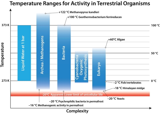
Figure 3. Examples of temperature ranges for different types of organisms, taken for species at the extreme ranges of survival in the laboratory.
To demonstrate their framework, they work through models for archaean life on Trappist 1e and Trappist 1f, cyanobacteria on the same 2 planets, methanogens (that would include archaea) in the subsurface of Mars, and the subsurface ocean of Enceladus.
Figure 4 below shows the simplified model for archaea on Trappist 1e. The values and standard deviations used for the priors are not all explained in the text. For example, the mean surface pressure is set at 5 Bar for illustrative purposes, as no atmosphere has been detected for Trappist-1e. The network model for the various modules that determine the viability of an archaean is mapped in a). Only 2 variables, surface temperature and pressure, determine viability of the archaean prokaryotes in the modeled surface temperature. In more sophisticated models, this would be a multidimensional plot perhaps using principal component analysis (PCA) to show a 3D plot. The various assumed (prior) and calculated (result) values and their assumed distributions are shown as charts in b). The plot of viability (1) and non-viability (0) for surface temperature and pressure is shown in the 3D plot c. The distributions indicate the probability of suitability of the habitat.
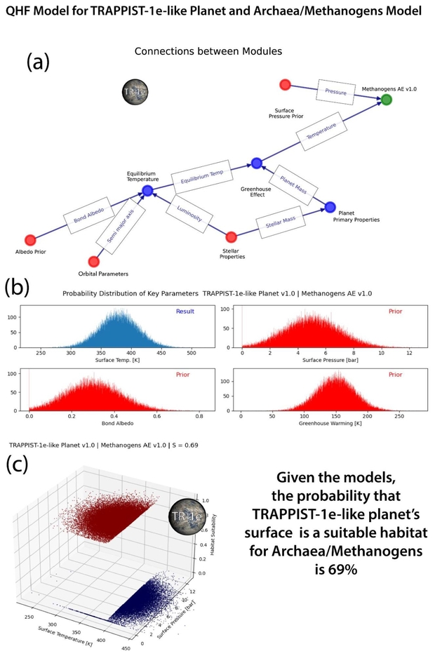
Figure 4. QHF assessment of the viability of archaea/methanogens in a modeled TRAPPIST-1e-like planet’s surface habitat. a: Connections between the model modules. Red are priors, blue are calculated values, green is the viability model. b: Relative probability distributions of key parameters. c: The distribution of calculated viability as a function of surface temperature and pressure. The sharp temperature cutoff at 395K separates the habitat as viable or not.
The examples are then tabulated to show the probabilities of different unicellular life inhabiting the various example worlds.
As you can see, the archaea/methanogens on Trappist 1f have the highest probability of being present inhabiting that world if we assume terrestrial life represents good examples. Therefore, Trappist 1f would be prioritized given the information currently available. If spectral data suggested that there was no water in Trappist 1f’s atmosphere, this would reduce, and possibly eliminate, this world’s habitability probability, and with it the probability of it meeting the requirement of archaean life and hence reducing the overlap in the habitability and life requirement terms to nil.
My Critique of the Methodology
The value of this paper is that it goes beyond the usual “Is the exoplanet habitable?” with the usual caveats about habitability that apply under certain conditions, usually atmospheric pressure and composition. The habitable zone (HZ) around a star is calculated for the range of distances from the star where, with an ideal atmosphere composition and density, on a rocky surface, liquid water could be found. Thus, early Mars, with a denser atmosphere, could be habitable [2], and indeed, the evidence is that water was once present on the surface. Venus might also once have been habitable, positioned at the inner edge of our sun’s HZ, before a runaway greenhouse made the planet uninhabitable.
The concept of NASA’s “Follow the water” mantra is a first step, but this paper then points out this is only part of the equation when deciding the priority of expending resources on observing a prospective exoplanet for life. The Earth once had an anoxic atmosphere, making Lovelock’s early idea that gases in disequilibrium would indicate life, which quickly became interpreted as free oxygen (O2) and methane (CH4), largely irrelevant during this period before oxygenic photosynthesis changed the composition of the atmosphere.
Yet Earth was living within a few hundred million years after its birth, with organisms that predated the archaea and bacteria kingdoms [4]. Archaea are often methanogens, releasing CH4 into the early atmosphere at a rate exceeding that of geological serpentinization. Their habitat in the oceans must have been sufficiently temperate, albeit some are thermophilic, living in water up to 122 centigrade but under pressure to prevent boiling. If the habitability calculations include the important variables, then their methodology offers a rigorous way to determine the probability of particular terrestrial life on a prospective exoplanet.
The problem is whether the important variables are included. As we see with Venus, if the atmosphere was still Earthlike, then it might well be a prospective target. Therefore, an exoplanet on the inner edge of its star’s HZ might need to have its atmosphere modeled for stability, given the age of its star, to determine whether the atmosphere could still be earthlike and therefore support liquid water on the surface.
However, there may be other variables that we have repeatedly discussed on this website. Is the star stable or does it flare frequently? Does the star emit hard UV and X-rays that would destroy life on the surface by destroying organic molecules? Is the star’s spectrum suited for supporting photosynthesis, and if not, does it allow or prevent chemotrophs to survive? For complex life, is a large moon needed to keep the rotational axis relatively stable to prevent climate zones and circulation patterns from changing too drastically? Is the planet tidally locked, and if so, can life exist at the terminator, as we have no terrestrial examples to evaluate? The Ramirez paper [3] includes his modeling of Trappist 1e, using the expected synchronization of its rotation and orbital period, resulting in permanently hot and cold hemispheres.
While the authors suggest that the analysis can extend beyond species to ecosystems, and perhaps a biosphere, we really don’t know what the relevant variables are in most cases. Unicellular organisms are sometimes easily cultured in a laboratory, but most are not. We just don’t know what conditions they need, and whether these conditions exist on the exoplanet. It may be that the equation variables may be quite large, making the analyses too unwieldy to be worth doing to evaluate the probability of some terrestrial life form inhabiting the exoplanet.
A further critique is that organisms rarely can exist as pure cultures except in a laboratory setting with ideal culture media. Organisms in the wild exist in ecosystems, where different organisms contribute to the survival of others. For example, bacterial biofilms often comprise different species in layers allowing for different habitats to be supported, from anaerobes to aerobes.
The analysis gamely looks at life below the surface, such as lithophilic life 5 km below the surface of Mars, or ocean life in the subsurface Enceladan ocean. But even if the probability in either case was 100% that life was present, both environments are inaccessible compared to other determinants of life that we can observe with our telescopes. This would apply to icy moons of giant exoplanets, even if future landers established that life existed in both Europan and Enceladan subsurface oceans.
What about exoplanets that are not in near circular orbits, but more eccentric, like Brian Aldiss’ fictional “Heliconia”? How to evaluate their habitability? Or circumbinary planets where the 2 stars are creating differing instellation patterns as the planet orbits its close binary?. Lastly, can tidally locked exoplanets support life only at the terminator that supports the range of their known requirements, such as Ramirez’ modeling of Trappist 1e?
An average surface temperature does not cover either the extremes, for example the tropics and the poles, nor that water is at its densest at 277K (4 °C), ensuring that there is liquid water even when the surface is fully glaciated above an ocean. Interior heat can also ensure liquid water below an icy surface, and tidal heating can contribute to heating even on moons that have exhausted their radioactive elements. If the Gaia hypothesis is correct, then life can alter a planet to support life even under adverse conditions, stabilizing the biosphere environment. The range of surface temperatures is covered by the Gaussian distribution of temperatures as shown in Figure 4 b.
Lastly, while the joint probability model with Monte Carlo simulation to estimate the probability of an organism or ecosystem inhabiting the exoplanet is a relatively computationally lightweight model, it may not be the right approach with more variables added to the mix. The probabilities may be disjoint with a union of different subsets of variables with joint probabilities. In other words, rather than “and” intersections of planet and organism requirement probabilities, there may be an “or” union of probabilities. The modeled approach may prove brittle and fail, a known problem of such models, which can be alleviated to some extent by using only subsets of the variables. Another problem I foresee is that a planet with richer observational data may score more poorly than a planet with few data-supported variables, simply due to the joint probability model.
All of which makes me wonder if the approach really solves the terminology issue to prioritize exoplanet life searches, especially if a planet is both habitable and potentially inhabited. It is highly terrestrial-centric, as we would expect, as we have no other life to evaluate. If we find another life on Earth, as posited by Paul Davies’ “Shadow Biosphere,” [4] this methodology could be extended. But we cannot even determine the requirements of extinct animals and plants that have no living relatives, but flourished in earlier periods on Earth. Which species survived when Earth was a hothouse in the Carboniferous, or below the ice during the global glaciations? Where were those conditions outside the range of extant species? For example, post-glacial humans could not survive during the Eocene thermal maximum.
For me, this all boils down to whether this method can usefully help determine whether an exoplanet is worth observing for life. If an initial observation ruled out an atmosphere like any of those Earth has experienced in the last 4.5 billion years, should the search for life be immediately redirected to the next best target, or should further data be collected, perhaps to look for gases in disequilibrium? While I wouldn’t bet that Seager’s ‘MorningStar’ mission to look for life on Venus will find anything, if it did turn up microbes in the acidic atmosphere’s temperate zone, that would add a whole new set of possible organism requirements to evaluate, making Venus-like exoplanets viable targets for life searches. If we eventually find life on exoplanets with widely varying conditions, with ranges outside of terrestrial life, would the habitat analyses then have to test all known life from a catalog of planetary conditions?
But suppose this strategy fails, and we cannot detect life, for various reasons, including instrumentation limits? Then we should fall back on the method I last posted on, which reduces the probability of extant life on an exoplanet, but leaves open the possibility that life will eventually be detected.
The paper is Apai et al (2025)., “A Terminology and Quantitative Framework for Assessing the Habitability of Solar System and Extraterrestrial Worlds,” in press at Planetary Science Journal. Abstract.
References
1. Schulze-Makuch, D. (2015) Astronomers Just Doubled the Number of Potentially Habitable Planets. Smithsonian Magazine, 14 January 2015.
https://www.smithsonianmag.com/air-space-magazine/astronomers-just-doubled-number-potentially-habitable-planets-180953898/
2. Seager, S. (2013) “Exoplanet Habitability,” Science 340, 577.
doi: 10.1126/science.1232226
3. Ramirez R., (2024). “A New 2D Energy Balance Model for Simulating the Climates of Rapidly and Slowly Rotating Terrestrial Planets,” The Planetary Science Journal 5:2 (17pp), January 2024
https://doi.org/10.3847/PSJ/ad0729
4. Tolley, A. (2024) “Our Earliest Ancestor Appeared Soon After Earth Formed” https://www.centauri-dreams.org/2024/08/28/our-earliest-ancestor-appeared-soon-after-earth-formed
5. Davies P. C. W. (2011) “Searching for a shadow biosphere on Earth as a test of the ‘cosmic imperative,” Phil. Trans. R. Soc. A.369624–632 http://doi.org/10.1098/rsta.2010.0235
A Sedna Orbiter via Nuclear Propulsion
When you’re thinking deep space, it’s essential to start planning early, at least at our current state of technology. Sedna, for example, is getting attention as a mission target because while it’s on an 11,000 year orbit around the Sun, its perihelion at 76 AU is coming up in 2075. Given travel times in decades, we’d like to launch as soon as possible, which realistically probably means sometime in the 2040s. The small body of scientific literature building up around such a mission now includes a consideration of two alternative propulsion strategies.
Because we’ve recently discussed one of these – an inflatable sail taking advantage of desorption on an Oberth maneuver around the Sun – I’ll focus on the second, a Direct Fusion Drive (DFD) rocket engine now under study at Princeton University Plasma Physics Laboratory. Here the fusion fuel would be deuterium and helium-3, creating a thermonuclear propulsion thruster that produces power through a plasma heating system in the range of 1 to 10 MW.
DFD is a considerable challenge given the time needed to overcome issues like plasma stability, heat dissipation, and operational longevity, according to authors Elena Ancona and Savino Longo (Politecnico di Bari, Italy) and Roman Ya. Kezerashvili (CUNY), the latter having offered up the sail concept mentioned above. See Inflatable Technologies for Deep Space for more on this sail. A mission to so distant a target as Sedna demands evaluation of long-term operations and the production of reliable power for onboard instruments.
Nonetheless, the Princeton work has captured the attention of many in the space community as being one of the more promising studies of a propulsion method that could have profound consequences for operations far from the Sun. And it’s also true that getting off at a later date is not a showstopper. Sedna spends about 50 years within 85 AU of the Sun and almost two centuries within 100 AU, so there is an ample window for developing such a mission. Some mission profiles for closer targets, such as Titan and various Trans-Neptunian objects, and other Solar System destinations are already found in the literature.
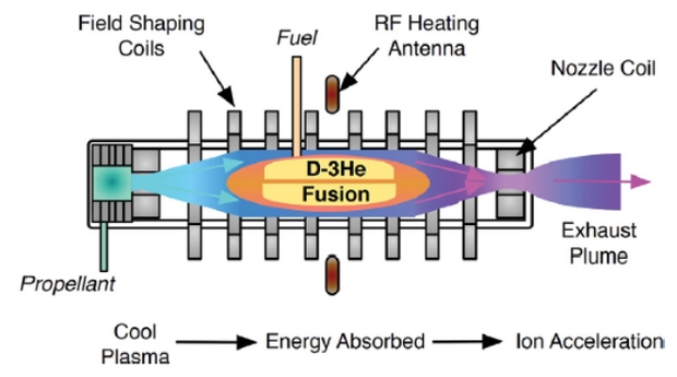
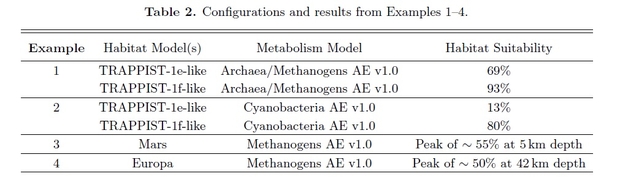
Image: Schematic diagram of the Direct Fusion Drive engine subsystems with its simple linear configuration and directed exhaust stream. A propellant is added to the gas box. Fusion occurs in the closed-field-line region. Cool plasma flows around the fusion region, absorbs energy from the fusion products, and is then accelerated by a magnetic nozzle. Credits [5].
The Direct Fusion Drive produces electrical power as well as propulsion from its reactor, and shows potential for all these targets as well as, obviously, more immediate destinations like Mars. What is being called a ‘radio frequency plasma heating’ method uses a magnetic field that contains the hot plasma and ensures stability that has been hard to achieve in other fusion designs. Deuterium and tritium turn out to be the most effective fuels in terms of energy produced, but the deuterium/helium-3 reaction is aneutronic, and therefore does not require the degree of shielding that would otherwise be needed.
The disadvantages are also stark, and merit a look lest we get overly optimistic about the calendar. Helium-3 and deuterium require reactor temperatures as much as six times higher than demanded with the D-T reaction. Moreover, there is the supply problem, for the amount of helium-3 available is limited:
The D-3He reaction is appealing since it has a high energy release and produces only charged particles (making it aneutronic). This allows for easier energy containment within the reactor and avoids the neutron production associated with the D-T reaction. However, the D-3He reaction faces the challenge of a higher Coulomb barrier [electrostatic repulsion between positively charged nuclei], requiring a reactor temperature approximately six times greater than that of a D-T reactor to achieve a comparable reaction rate.
So what is the outline of a Direct Fusion Drive mission if we manage to overcome these issues? The authors posit a 1.6 MW DFD, working the numbers on the Earth escape trajectory, interplanetary cruise (a coasting phase) and final maneuvers at target. In an earlier paper, Kezerashvili has shown that the DFD option could reach the dwarf planet Eris in 10 years. The distance of 78 AU matches with Sedna’s perihelion, meaning Sedna itself could be visited in roughly half the time calculated for any other propulsion system considered.
Bear in mind that it has taken New Horizons 19 years to reach 61 AU. DFD is considerably faster, but notice that the mission outlined here assumes that the drive can be switched on and off for thrust generation, meaning a period of inactivity during the coasting phase. Will DFD have this capability? The authors also evaluate a constant thrust profile, with the disadvantage that it would require additional propellant, reducing payload mass.
In the thrust-coast-thrust profile, the authors’ goal is to deliver a 1500 kg payload to Sedna in less than 10 years. The authors calculate that approximately 4000 kg of propellant would be demanded for the mission. The DFD engine itself weighs 2000 kg. The launch mass bumps up to 7500 kg, all varying depending on instrumentation requirements. From the paper:
The total ∆V for the mission reaches 80 km/s, with half of that needed to slow down during the rendezvous phase, where the coasting velocity is 38 km/s. Each maneuver would take between 250 and 300 days, requiring about 1.5 years of thrust over the 10-year journey. However, the engine would remain active to supply power to the system. The amount of 3He required is estimated at 0.300 kg.
The launch opportunities considered here begin in 2047, offering time for DFD technology to mature. As I mentioned above, I have not developed the solar sail alternative with desorption here since we’ve examined that option in recent posts. But by way of comparison, the DFD option, if it becomes available, would enable much larger payloads and the rich scientific reward of a mission that could orbit its target rather than perform a flyby. Payloads of up to 1500 kg may become feasible, as opposed to the solar sail mission, whose payload is 1.5 kg.
The two missions offer stark alternatives, with the authors making the case that a fast sail flyby taking advantage of advances in miniaturization still makes a rich contribution – we can refer again to New Horizons for proof of that. The solar sail analysis with reliance on sail desorption and a Jupiter gravity assist makes it to Sedna in a surprising seven years, thus beating even DFD. The velocity is achieved by coating the sail with materials that are powerfully ‘desorbed’ or emitted from it once it reaches a particular heliocentric distance.
Thus my reference to an ‘Oberth maneuver,’ a propulsive kick delivered as the spacecraft reaches perihelion. Both concepts demand extensive development. Remember that this paper is intended as a preliminary feasibility assessment:
Rather than providing a fully optimized mission design, this work explores the trade-offs and constraints associated with each approach, identifying the critical challenges and feasibility boundaries. The analysis includes trajectory considerations, propulsion system constraints, and an initial assessment of science payload accommodation. By structuring the feasibility assessment across these categories, this study provides a foundation for future, more detailed mission designs.
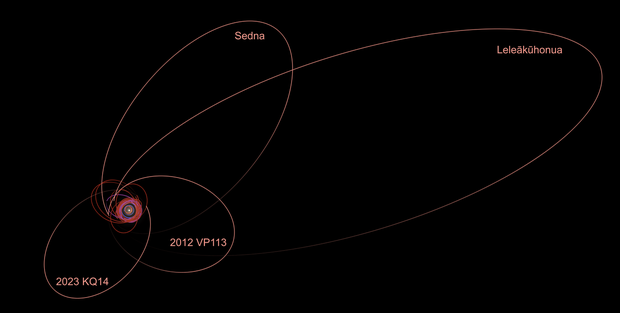
Image: Diagram showing the orbits of the 4 known sednoids (pink) as of April 2025. Positions are shown as of 14 April 2025, and orbits are centered on the Solar System Barycenter. The red ring surrounding the Sun represents the Kuiper belt; the orbits of sednoids are so distant they never intersect the Kuiper belt at perihelion. Credit: Nrco0e, via Wikimedia Commons CC BY-SA 4.0.
The boomlet of interest in Sedna arises from several factors, including the fact that its eccentric orbit takes it well beyond the heliopause. In fact, Sedna spends only between 200 and 300 years within 100 AU, which is less than 3% of its orbital period. Thus its surface is protected from solar radiation affecting its composition. Any organic materials found there would help us piece together information about photochemical processes in their formation as opposed to other causes, a window into early chemical reactions in the origin of life. The hypothesis that Sedna is a captured object only adds spice to the quest.
The paper is Ancona et al., “Feasibility study of a mission to Sedna – Nuclear propulsion and advanced solar sailing concepts,” available as a preprint.
JWST Catch: Directly Imaged Planet Candidate
We have so few exoplanets that can actually be seen rather than inferred through other data that the recent news concerning the star TWA 7 resonates. The James Webb Space Telescope provided the data on a gap in one of the rings found around this star, with the debris disk itself imaged by the European Southern Observatory’s Very Large Telescope as per the image below. The putative planet is the size of Saturn, but that would make it the planet with the smallest mass ever observed through direct imaging.
Image: Astronomers using the NASA/ESA/CSA James Webb Space Telescope have captured compelling evidence of a planet with a mass similar to Saturn orbiting the young nearby star TWA 7. If confirmed, this would represent Webb’s first direct image discovery of a planet, and the lightest planet ever seen with this technique. Credit: © JWST/ESO/Lagrange.
Adding further interest to this system is that TWA 7 is an M-dwarf, one whose pole-on dust ring was discovered in 2016, so we may have an example of a gas giant in formation around such a star, a rarity indeed. The star is a member of the TW Hydrae Association, a grouping of young, low-mass stars sharing a common motion and, at about a billion years old, a common age. As is common with young M-dwarfs, TWA 7 is known to produce strong X-ray flares.
We have the French-built coronagraph installed on JWST’s MIRI instrument to thank for this catch. Developed through the Centre national de la recherche scientifique (CNRS), the coronagraph masks starlight that would otherwise obscure the still unconfirmed planet. It is located within a disk of debris and dust that is observed ‘pole on,’ meaning the view as if looking at the disk from above. Young planets forming in such a disk are hotter and brighter than in developed systems, much easier to detect in the mid-infrared range.
In the case of TWA 7, the ring-like structure was obvious. In fact, there are three rings here, the narrowest of which is surrounded by areas with little matter. It took observations to narrow down the planet candidate, but also simulations that produced the same result, a thin ring with a gap in the position where the presumed planet is found. Which is to say that the planet solution makes sense, but we can’t yet call this a confirmed exoplanet.
The paper in Nature runs through other explanations for this object, including a distant dwarf planet in our own Solar System or a background galaxy. The problem with the first is that no proper motion is observed here, as would be the case even with a very remote object like Eris or Sedna, both of which showed discernible proper motion at the time of their discovery. As to background galaxies, there is nothing reported at optical or near-infrared wavelengths, but the authors cannot rule out “an intermediate-redshift star-forming [galaxy],” although they calculate that probability at about 0.34%.
The planet option seems overwhelmingly likely, as the paper notes:
The low likelihood of a background galaxy, the successful fit of the MIRI flux and SPHERE upper limits by a 0.3-MJ planet spectrum and the fact that an approximately 0.3-MJ planet at the observed position would naturally explain the structure of the R2 ring, its underdensity at the planet’s position and the gaps provide compelling evidence supporting a planetary origin for the observed source. Like the planet β Pictoris b, which is responsible for an inner warp in a well-resolved—from optical to millimetre wavelengths—debris disk, TWA 7b is very well suited for further detailed dynamical modelling of disk–planet interactions. To do so, deep disk images at short and millimetre wavelengths are needed to constrain the disk properties (grain sizes and so on).
So we have a probable planet in formation here, a hot, bright object that is at least 10 times lighter than any exoplanet that has ever been directly imaged. Indeed, the authors point out something exciting about JWST’s capabilities. They argue that planets as light as 25 to 30 Earth masses could have been detected around this star. That’s a hopeful note as we move the ball forward on detecting smaller exoplanets down to Earth-class with future instruments.
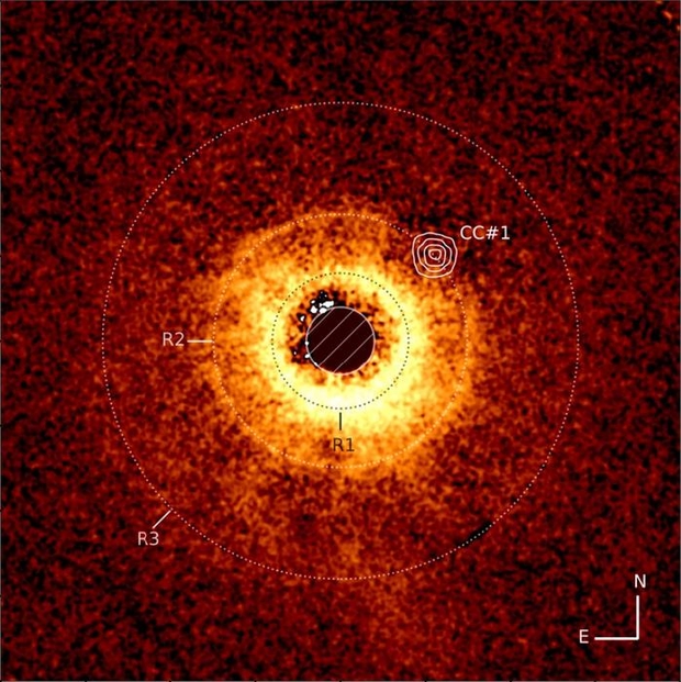
Image: The disk around the star TWA 7 recorded using ESO’s Very Large Telescope’s SPHERE instrument. The image captured with JWST’s MIRI instrument is overlaid. The empty area around TWA 7 B is in the R2 ring (CC #1). Credit: © JWST/ESO/Lagrange.
The paper is Lagrange et al., “Evidence for a sub-Jovian planet in the young TWA 7 disk,” Nature 25 June 2025 (full text).
Addendum: I’ve just become aware of Crotts et al., “Follow-Up Exploration of the TWA 7 Planet-Disk System with JWST NIRCam,” accepted for publication at Astrophysical Journal Letters (preprint). From which this:
…we present new observations of the TWA 7 system with JWST/NIRCam in the F200W and F444W filters. The disk is detected at both wavelengths and presents many of the same substructures as previously imaged, although we do not robustly detect the southern spiral arm. Furthermore, we detect two faint potential companions in the F444W filter at the 2-3σ level. While one of these companions needs further followup to determine its nature, the other one coincides with the location of the planet candidate imaged with MIRI, providing further evidence that this source is a sub-Jupiter mass planet companion rather than a background galaxy. Such discoveries make TWA 7 only the second system, after β Pictoris, in which a planet predicted by the debris disk morphology has been detected.
Follow with RSS or E-Mail
