Wes Kelly has pursued a lifetime interest in flight through the air, in orbit and even to the stars. Known on Centauri Dreams as ‘wdk,’ Wes runs a small aerospace company in Houston (Triton Systems,LLC), founded for the purpose of developing a partially reusable HTOL launch vehicle for delivering small satellites to space. The company also provides aerospace engineering services to NASA and other customers, starting with contracts in the 1990s. Kelly studied aerospace engineering at the University of Michigan after service in the US Air Force, and went on to do graduate work at the University of Washington. He has been involved with early design and development of the Space Shuttle, expendable launch systems, solar electric propulsion systems and a succession of preliminary vehicle designs. With the International Space Station, he worked both as engineer and a translator or interpreter in meetings with Russian engineering teams on areas such as propulsion, guidance and control. In today’s essay, Wes ponders our view of the nearest stars and how, during the course of his career, we have looked at exoplanets and the question of habitability.

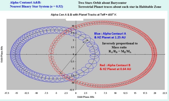
Figure 1. Elliptical traces of Alpha Centauri stars A & B about their barycenter with planets in the habitable one (HZ) for each star based on stellar effective temperature equivalent to Earth.

Now that Centauri-Dreams has been around for about fifteen years, can you remember what it was like before it came along? Or for that matter, arrival of the perception of Alpha Centauri as a place rather than a bright star low on the Northern Hemisphere horizon? In the matter of speculations about the nearest of stars, there was a time when all science could say was that these were the closest and those in the binary pair were quite similar to our own sun. That era, starting about 1840, has resulted in us looking to the system for an Earth analog or two, perhaps shaving off centuries from potential migration treks our descendants might require to arrive at one. Exotic too, if they exist, what with A, B and Proxima all in the sky. But we still haven’t resolved that question of existence.

The viability of Earth-like Alpha Centauri planets had fascinated me enough back in the 1980s to simulate their orbital tracks (Figure 1), these along with other binary system planets. When Doppler detection of Jupiter sized planets started to occur in the 1990s, I expanded the simulations to include those planets’ effects as well, examining their influence on putative habitable zone (HZ) terrestrial sized planets nearby them. I participated in at least one early exoplanet conference (“Planet Formation in the Binary Environment”, June 1996, Stony Brook, NY) and then a few astrodynamics and planetary science conferences before and after. When there were recent reports of Jovian planets on highly eccentric paths, one orbiting HR-5183 (“Gas Giants on Eccentric Orbits: ‘Wrecking Balls’ for the Inner System?”, Paul Gilster, 06 November 2019), it brought back memories, plus stimulus to review exoplanet analyses and musings over the years.

To give a quick summary, if HZ terrestrial planets exist in binary systems, their patterns of motion are similar to ours, but distorted to varying degrees. In some cases, such as the Dog Star (Sirius A – Figure 2), there is simply not enough room for them to survive intact for thousands of years (Figure 3). In others, conditions are exotic and dynamic enough to raise questions of whether the planets could form in the first place. But then we have found that the nature of surviving planetary systems around other stars can be so exotic, that we should not be too quick to write binary system planets off. The influence of large planets on careening paths has to be considered too. In the days before Centauri Dreams, initial discoveries often were the wrecking balls in the inner systems; or else outer planet gas giants on eccentric paths. But for the most part terrestrial planets remained invisible until high performance transit methods could be devised in this, the next century (e.g. Corot, Kepler and TESS observatories).

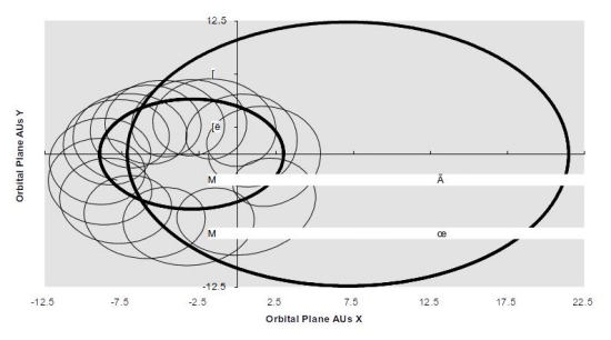
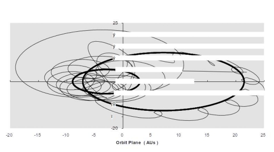
Figure 2. Sirius A and B, A with A1 Planetary Track at T_eff = 400° K, Sirius A is the smaller diameter bold ellipse track. Planet shifts to Sirius B orbit before ejection. Integration for 25,000 days, a* = 30.26 AUs, e* = .50, P* = 49.9 yrs, R_o = 4.88 AU, T_eff = 400° K Stellar Mass: M_A = 2.35, M_B = 0.95, Luminosity: L_A = 23, L_B = .00229 (Solar Units).

Orbit Plane (AUs)

Figure 3. Sirius A and B, A with planetary track prior to ejection: Capture by B prior to ejection. Sirius A is the smaller diameter bold ellipse track. Planet shifts to Sirius B orbit before ejection.

As for reflection, for a start, what would Centauri Dreams be like without the internet? By the time the Centauri system was designated a close neighbor in the 1840s, researchers could coordinate via telegraph at least. But even in the 1970s, there was still much isolation for people concerned with “exoplanets”, a term yet to be coined. There were no databases as yet on a world-wide web. The two quirky research journals you were most likely to find something about what constituted exoplanet research so far: Icarus and the Journal of the British Interplanetary Society. You could inform yourself If you subscribed long enough ($$) or you were near the right library. With the Astronomical Journal, you would just have to stay tuned… to read about negative results. Decades ago, you could not simply google search exoplanet studies; thus, communication had considerable lag even here on Earth. For example, in the 1970s, you could examine engineering details of the BIS Daedalus Project space probe targeted to Barnard’s Star, the presumed Red Dwarf host to several large planets based on tenuous slow data rate astrometric studies appearing in the Astronomical Journal in the 1970s. The picture was later refuted. Daedalus was not necessarily re-targeted to Centauri, because there were still no known planets beyond the solar system. Information was not closely held, but not easily generated or disseminated either.

When I started simulating planetary motions in the 1980s, the scientific community still kept stars and planets compartmentalized rather tightly, the latter simply as a study of the solar system. Yet back then for many of the visitors and contributors to this website, no doubt there were dreams or speculations about Alpha Centauri. And for a number of us reading science fiction decades back, if adventure ranged beyond the solar system, Mars and Martians, now and then there was a book or video episode set on a planet around this closest system of stars.

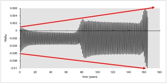
Figure 4. ? Centauri A planetary orbit perturbation over 160 years or 2 stellar revolutions. R_o = 1.2468 AU, T_eff = 400° K, period = 486 days, P* = 79.9 years.

Among the first I encountered was in grade school, Lee Correy’s (G. Harry Stine’s) Starship through Space. I wish I could remember how the hyperspace problem was solved… But with Correy’s dtailed account of heading back to Earth from Mars to join the big expedition, I was ready to believe anything. There was also a late entry into the “Tom Corbett Space Cadet” series, treated by publishers like a cousin or descendant of Tom Swift. Danger in Deep Space read suspiciously like the Navy planning a World War II island invasion or beach head. Tom, Roger and Astro were underclassmen of a future spatial Naval Academy and I suspect the author had been an ensign once too.

Another Centauri tale cycle I encountered early on was via the city library system’s bookmobiles: Andre Norton’s stories with titles like The Stars Are Ours. If building the Empire State Building was an accomplishment in the depths of the Depression, imagine Norton’s intrepid leader Dalgard Nordiss rallying the scientific establishment for interstellar migration after nuclear war. No? Maybe the survivors might have wanted a word or two with them before they left? The stories had other idiosyncrasies.

As for the pulp magazine interstellar stories though, Alpha Centauri did not seem to figure very prominently against a galaxy wide locale selection. But at about the time I started examining stability of planets in binary star systems, Jerry Pournelle and Larry Niven wrote a novel (Footfall) with the opposite tack: “exo-pachyderms” from the Centauri system had arrived here for a hostile takeover. They had perfected Robert Bussard’s concept for a space drive, not that that was much consolation.

These musings come atop those of antiquity. Lucretius and other ancients believed that there were other worlds, though I am not sure where they meant. And early 17th century traveling monk Giordano Bruno believed that stars were actually suns with planets, possibly drawing this inference from those Greek and Roman atomists writing a millennium and a half earlier. If not, then how?

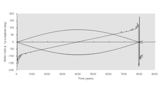
Figure 5. Centauri A planet (?R/R_o) max, min and ?_p over ~100 stellar revolutions. R_o = 1.2468 AU, T_eff = 400° K, P= 486 days, P*=79.9 years (terrestrial). Eccentricity cycles with 180° Shift of nodes periastron-astron. For particular case, ?R/R₀ max & min + & – 0.08 at ~4,000 Earth Years.

But the transformation of immovable heavenly ceiling lights into objects similar to the sun is not so clearly demarcated in scientific history as Copernicus, Kepler and Galileo’s arguments and evidence for this particular set of planets going around this particular sun. First, it was necessary to demonstrate stellar movements in the celestial sphere at all with trigonometric measurements from opposite ends of Earth’s orbit around the sun (parallax). That itself took decades. After 61 Cygni in the northern hemisphere was determined by mathematician and astronomer F. W. Bessel of function fame (1838) to be about eleven light years away, search in the southern hemisphere revealed Alpha Centauri as even closer (4.3). And these observations rested on the ability to discern less than an arc second shift in the sky. So centuries after the public came to think of Mars and Venus as close neighbors, it finally had some stars to associate as neighbors too, just a few hundred thousand times as far away.

Then for detection of planets, the next step would be to show that a star and planet moved around a common center of mass (a barycenter). The sun’s shift due to Jupiter is a circular path about their common center of mass about 1000th the width of Jupiter’s orbit around the sun (Figure 6). And it had been established that stars projected on the celestial sphere could project paths due to seen or unseen stellar partners (Figure 7) – the first “wrecking balls”). The trouble was, stars were just so much more massive than planets like the Earth. In our local and earthly case it is about 330,000 to 1, Sun’s favor. Astrometric measurements of planets around any star in the first half of the 20th century looked headed for fiasco or bust on account of measurement low signal to noise ratios or eventual systematic errors or biases. Doppler detections due to induced stellar motions had similar issues – until the 1990s.

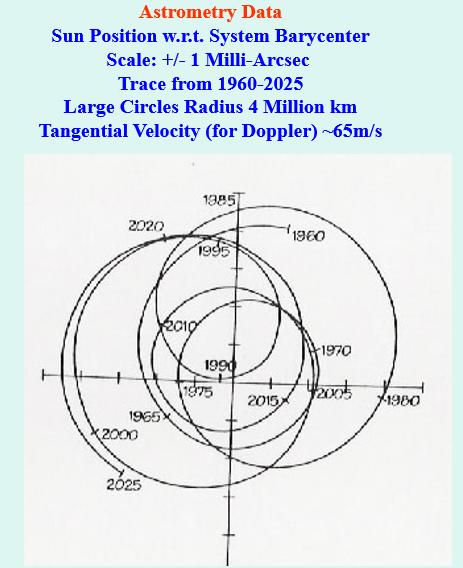
Figure 6. The Little Green Men astrometric case for the existence of Jupiter and Saturn. Solar wanderings in celestial sphere Due to Jupiter-Sun and other (Cumulative). Barycenter rotations from the other planets’ view from 10 parsec distance over “North Pole” of ecliptic plane. 1 Parsec = 3600*180/? = 206,264.8 astronomical units tangential velocity for observation on ecliptic plane (Doppler) ~65 m/s due to Jupiter.

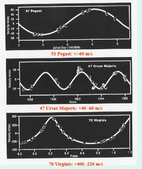
Figure 7. Stellar velocity shifts for early exoplanet detections from Doppler readings. Jupiter magnitude Doppler shifts (51 Pegasi and 47 Ursae Majoris) and more (70 Virginis). 51 Pegasi over days, the others over years and 70 Virginis significantly eccentric.

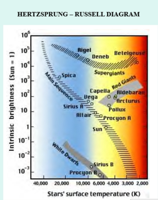
Figure 8 The variety of stars based on the Herzsprung-Russell diagram. “X-axis” based on surface temperature. “Y-axis” solar scale luminosity or intrinsic brightness. The Main Sequence of hydrogen fusion burning inversely proportional to mass. Stellar Main Sequence brightness as a function of mass to the third or fourth Power.

Once stars were identified as suns, there remained another problem, associated with the growing understanding of stellar structure, evolution and origin, their temperatures and brightness (Figures 8 and 9). Stars coalesced out of clouds of gas. And these condensing gas clouds from which they formed: they appeared to have a minimum mass (i.e., Jeans mass limit), still a hefty solar fraction. It was about the same mass as that required for the ignition of hydrogen fusion, about 8 percent of solar mass. Coincidence? This did not bode well for brown dwarfs, for one, but the idea certainly knocked the chair out from under arguments for exoplanets, a term that still needed to be coined. Having been around an astronomy department where there were accomplished researchers of all manner of stellar development and structure back in the 1970s, these points were drilled home.

But in the 1970s and 80s, there was at least one source of hope: Infra-red observatories and results were coming on line. Among the structures detected with new instruments were “circumstellar” disks or CSDs. Notably, the Infrared Astronomical Satellite (IRAS) had imaged one surrounding the young southern hemisphere star Beta Pictoris. This had possibilities… More young stars featured them. Perhaps a short lived but significant phenomenon which could lead to something? If the spatial distribution could not be discerned directly, many young stars had a characteristic infra-red departure from their black body spectra. Orbital observatories with ultraviolet sensitivities (ROSAT) were pointing out some interesting related features too. Spectral features suggested young stars were surrounded by rings of heated dust and gas and there could be significant coalescence.

But for the most part, if ad hoc solar system explanations such as a close passage of another star did not explain the existence of planets, it had been largely argued by many stellar astronomers that planets were a rare off-shoot of stellar evolution. Like biological life, multi-cellular organisms, intelligence and consciousness are suspected to be today, barring something like a post Kepler space observatory moment for any of these traits. Since the 1960s newspapers and Scientific American articles have cited the Drake equation regarding likelihood for extraterrestrial life. Sometimes this factorial equation suggested that planets and maybe even “Earths” proliferated across the galaxy almost as much as stars. The Drake equation, depending on assumptions, could give; but with further reflection it also could take away. At least on corridors where stellar astronomers congregated.

===========

The Drake Equation

N= R? f_P n_e f_L f_I f_C L

N = the number of civilizations in our galaxy with which communication might be possible

R? = the average rate of star formation in our galaxy

f_P = fraction of those stars that have planets

n_e = average number of planets that can potentially support life per star that has planets

f_L = fraction of planets that could support life that actually develop life at some point

f_I = fraction of planets with life that actually go on to develop intelligent life (civilizations)

f_C = fraction of civilizations that develop technology releasing detectable signs of their existence

L = the length of time for which such civilizations release detectable signals into space.

===========

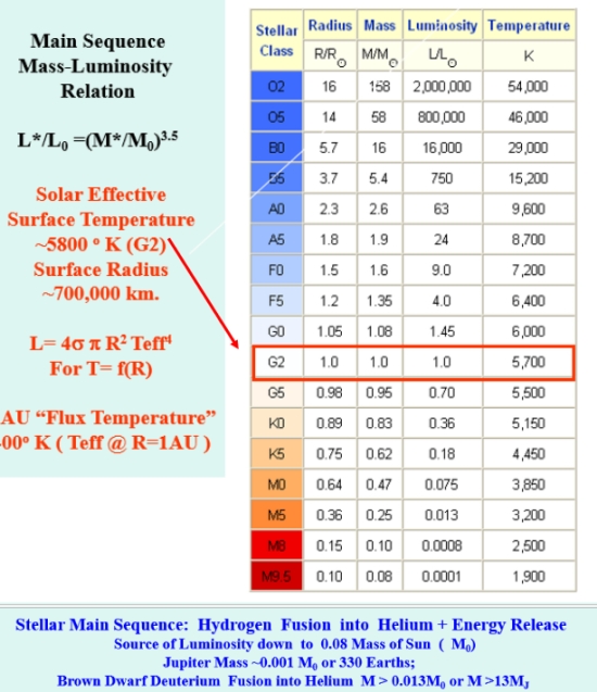
Figure 9. Stellar main sequence classifications and characteristics provide a basis for predicting habitable zones for terrestrial planets: Locating radii of equivalent 400° K effective temperature.

Beside those objections regarding coalescing clouds in the interstellar medium decades back, there are other relations between the number of stars and number of planets to consider. The majority of stars in the galaxy are tied up in binary systems of varying distance and eccentricity. Moreover, as we have discovered since, planets within stellar systems vary in mass beyond that of Jupiter and they can follow eccentric paths too. Getting an assessment of how many Earth-like planets exist does not stop at analyzing stellar binaries, but extends to several categories. Hats off to Bullwinkle Moose and Rocky Squirrel, who circa 1960 introduced many young TV watchers to new concepts with their own cartoon clarion call “the Restricted Elliptic 3-body Problem” (RE3BP). For our purposes we can divide the problem into several categories.

1. Stellar binary systems of Solar System dimensions with significant eccentricity, crowding the habitability zone (a ring with inner and outer radii). Examples or cases: Alpha Centauri, Procyon, Sirius…

2. Close stellar binaries providing a bi-polar gravitational and thermal source to the habitable zone.

3. Jovian mass planets or brown dwarfs with semi-major axes external to the habitable zone, particularly those with non-zero eccentricities.

4. Jovian mass planets or Brown Dwarfs in or passing through the habitable with non-zero eccentricities.

5. Binary systems in which the habitable planet is a satellite of the Jovian planet or brown dwarf in a habitable zone.

More can be conceived, but this is enough for now. These distinctions help focus on orbital stability if not necessarily habitability, also a function of local temperatures.

In the first category, there have been some possible or probable observational detections of Centauri planets, but nothing so far related to Procyon or Sirius. And our dynamic analysis gives little chance of habitable planets existing near Sirius, with the case surrounding Procyon dicey. We have examined a few close binary cases (e.g., Castor) which did not pose problems (category 2). In categories 3 and 4, we examined the early Doppler detections of Jovian mass planets at 47 Ursae Majoris and 70 Virginis for their effect on putative terrestrial planets in their habitable zones or else as satellites of those bodies.

Since the data for 47 Ursae Majoris and 70 Virginis planets were based on Doppler measurements, the mass times sine of inclination issue has to be addressed (m_PL sin i). If the line of sight to the star runs through the planet’s orbital plane, its inclination is considered to be perpendicular (90 degrees) to that of the fictitious background celestial sphere. But Doppler data represents only sin(i) projections of velocity, so the in-plane orbital velocity of the primary would be larger, and the planet more massive.

Also, at this time, it is convenient to make the distinction between 2-body conic eccentricity “e” and the variations we will observe for very perturbed orbits tracing a path of 360 degrees around their primaries. If we can establish a reference orbital radius (R₀) for a near circular orbit, then (R-R₀)/R₀ provides a non-dimensional ?R/R₀ variation of radius, whether the orbit follows a truly elliptical path or not, The the angle of orbital passage from the periapse or closest point to the primary, shall we say, just might present a “not so true anomaly” angle if the elliptical path is distorted. And if an elliptical flight path is distorted, then predicting flight times between two angles or radii becomes much more complicated. In simulation, generally, I would watch for local max and min values over a nominal orbital period, tag the times and record it and other parameters in plot files. Hence the plots shown.

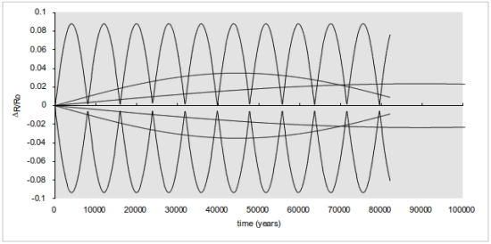
Figure 10. RE3BP Planetary orbit perturbations for Earth, Mars and Centauri A planet, eccentricity periods in descending order. Current Earth and Mars eccentricity .016722 and .093377.

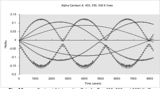
Figure 11. ? Centauri A integration data for T_eff=400, 350 and 300° K (R_o=1.2468, 1.6825, 2.2165 AU). Transition to instability and ejection from radii 2.0 to 2.75 (~T_eff = 225° K)

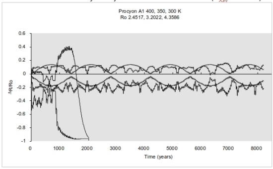
Figure 12. Procyon A1 integration data for T_eff=400, 350 and 300° K (R_o=2.4517, 3.2022, 4.3586 AU). Stable cycle for 400° K, ragged pattern for 350° K, de-orbit into primary for 300° K case.

“Call me Ishmael”

Most of my professional career has been in aerospace engineering. It would be an exaggeration to say that I have straddled it and astronomy or astrophysics, but now and then something interesting would come my way through assignments, or I have tinkered with concepts resulting from following events or mulling topics from graduate studies. With aerospace, in the 1970s, I became involved in detailed simulations of the Space Shuttle and its many phases of flight, main frame style; and in the 1980s I began to look at other vehicles hosted on smaller and smaller computers taking away some lessons learned, eventually to personal computers, an idea that seemed like a delight. One particular simulation in the mid-1980s that I had developed in that environment was for a proposed low thrust orbital maneuver vehicle deploying the Hubble Space Telescope from the Space Shuttle in a low orbit to a higher orbit where the telescope would operate. But the main points were to consider the so-called finite burn and to model all the maneuvers that deployed the telescope and retrieve the Orbital Maneuver Vehicle (there was only supposed to be one article). I mention this for two reasons:

1. It was necessary to have a means to integrate motion numerically in a variety of terrestrial gravitational models: the uniform gravity field and some of the approximations of the gravity field accounting for Earth’s oblateness and other irregularities and then to compare. Terrestrial gravitation forces produce accelerations; cumulative with time, velocity changes; velocity cumulative with time, distance changes.

2. It was this body of code which I cut, spliced and revised for stellar binary simulations looking at well known nearby binary systems and (later) subsequent strange systems with closely bound Jupiter mass planets, discovered with the first successful Doppler studies for exoplanets. These systems had different gravitational fields as well due to mass and two body binary eccentricity. As perceived by the third body, you might say that they varied with time in a manner we are not accustomed to here on Earth.

The approach to integration could have proceeded in a number of ways. One was to assume masses and initial paths (position and velocity) for the three objects and let the integration scheme sum the forces, accelerations, velocities and positions. The alternative was to assume that the two principal objects proceeded on their fixed paths around their center of mass (barycenter) and the third body was acted on by their positions and forces of attraction. The reciprocal force could be ignored, just as we often do with artificial satellites with Earth and sometimes even the Moon itself. But a difference from heliocentric or Earth centered motion is that the two principal objects are in very elliptical paths inversely proportional to their ratios of mass around their center of mass or barycenter (e.g., Figures 1 and 2). Their close approach and most distant points are at opposite sides of the barycenter and always on a line through it. For a planet to orbit one or the other binary star, it has to be within the star’s sphere of influence, but it has to be more complicated than the criteria described for our solar system.

While the terrestrial spacecraft integrations were usually in steps of seconds, the binary star systems were usually incremented in days. Their gravitational constants were based on their mass with respect to the sun ( ~ 0.08 < M_SUN < 3.0 ). If a conic such as an ellipse is defined, there is an iterative convergent solution to the problem of distance from the focal center with respect to time, converging quickly enough. Series methods might be needed for highly eccentric systems. The inverse, time of flight to a specific radial distance would have been more intractable. But saying this, depending on when the studies were undertaken, exploration of star systems was limited by the computing power available at a given time. When this effort began, PCs were limited to Intel 8087 chips and corresponding mini-computer technologies. Nonetheless, what constituted an overnight run became longer and longer calculations.

Since I did not know where these studies would take me with the individual star systems, Alpha Centauri A initial results looked very alarming (Figure 4). Increasing eccentricity with every 79.98 year binary orbit suggested that planets would end up burning up like star grazing comets if the trend went on in linear fashion. It turned out that as the line of nodes (periastron and apoastron) rotated 180 degrees in the celestial sphere or with respect to the binary system axis, the trend reversed. Whether it was conservative or not, at least it appeared to be within the limits of double precision calculations. Figure 4 above indicates that the initial Alpha Centauri A test case experienced an 8000 earth year cycle of eccentricity oscillation based on the restricted elliptic 3-body problem so posed. As the initial circular radial distance from the primary was changed for various control volume temperatures, the eccentricity cycle increased in frequency (and magnitude) with lower temperatures. Beyond 3 AUs, the terrestrial planet in orbit around A would not remain for long. Procyon and Sirius were investigated in a similar fashion. Since the “primary” stars are so bright and their secondaries, the white dwarfs are so close, Procyon and Sirius posed tighter and tighter constraints on HZ stability. For Sirius A denizens (remember the Visitors in “V”? … Sorry) I saw no original home.

The Sun-Jupiter system was also used to examine its influence on Earth and Mars. The eccentricity cycles are shown to scale in Figure 10. In actuality, other planets such as Saturn would have secondary or tertiary effects on these cycles and these would not be the sole explanations for climate variations. Planetary rotational axes tend to precess as well over periods of thousands of years. For the earth, the 23.5 degree inclination cuts a circle in the celestial sphere over about 25,000 years.

Each star has a brightness or luminosity which can be looked at as a sum of its radiation over an entire spectrum with an approximate black body distribution. Stars burning hydrogen into helium burn more intensely with mass in a third or fourth power relation (L (M) ~ M^3.5), but radius increases not so sharply. If we consider the sun as a 700,000 km radius object with a 5800 degree Kelvin surface temperature, then if it were expanded to 1 Astronomical Unit radius, the effective surface temperature would be about 400 degrees Kelvin. Earth is not that temperature due to a number of heat transfer considerations: its reflectance, the fact that only one hemisphere is illuminated at a time and its atmospheric greenhouse. Freezing water is about 273 Kelvin, so its mean temperature is closer to 300 degrees. But since both the planet and the star have thermodynamic differences, I prefer to model with planets by setting their radii at control volume temperature radii similar to the one above. If a star has more ultraviolet or infrared radiation due to higher or lower surface temperatures, then it might make sense testing stability at temperatures below and above the control volume temperature (350°, 400°, 450° K…) we would expect for a star and planet identical to Earth.

Giants Planets on the Inside Lane and Out

Now remember the wrecking ball planets? The early exoplanet examples 47 Ursae Majoris B and 70 Viriginis B were spectroscopic Doppler cases which had mass uncertainties associated with them. Detecting a periodic radial velocity component in their primary stars provided most of the evidence for their existence. If these two massive planets or brown dwarfs were in the line of sight of the observer, their inclination (i) for our purposes would be 90 degrees. But if this were exactly so, we would likely witness their transits across the faces of their stellar primaries with a dip in brightness as well. So far, we have not, which leaves the other 89 degrees or so as suspect. The two bodies, if in line of sight, were estimated at 2.3 and 6.8 jovian masses respectively. With a 45 degree inclination their masses would increase by about 40 percent. Thresholds for deuterium and hydrogen fusion at 13 and 70 Jupiter masses (M_J) respectively, raising the prospect of 70 Virginis B being a brown dwarf which had “burned” deuterium.

It is easy to confuse the features of these two early exoplanet systems since they both involve planets as large or larger than Jupiter in what we consider the domain of the terrestrial planets. But in the case of 70 Virginis B, its location is near the inner boundary of a HZ similar to Earth’s, while with 47 Ursae Majoris B, it is on the outer edge. There is considerable eccentricity associated with 70 Vir B, but not with 47 U Maj B.

Even in this era of several thousand planet detections owing mainly to the Kepler observatory and stellar transits, most planets detectable are larger than the Earth, which begs the question of whether Jupiters or Neptunes could harbor satellites like the large planets of our own system; perhaps even larger satellites than the ones we are familiar with thus far. But these large Jovian planets also have more eccentric orbits than our solar system examples, a characteristic 70 Virginis B seemed to announce with its detection. So despite the fact that its position did not bode well for life, I examined the effect of having a close satellite in orbit around a high eccentricity planet. In addition, and as usual, I also looked at an HZ terrestrial planet orbiting at about 1.73 AU semi major axis. And beside examining the nominal or minimum mass case for 70 Virginis B, I looked at values for masses based on shifts of orbital plane from the line of sight.

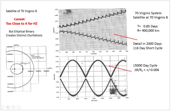
Figure 13. Satellite of Jovian planet 70 Virginis B, Distinct from planet in orbit around 70 Virginis A. Planet and satellite are close to 70 Vir A, not considered within HZ. Analysis shows oscillatory effects on satellite of eccentric binary systems with Jupiter-Sun mass.

With 70 Virginis B so close to its sun, there would be little prospect for life on a satellite, but Figure 13 shows an elaborate jitter that should keep it active in a geophysical sense. The satellite was placed in a 400,000 km radius orbit about B, a distance similar to the Moon’s distance from Earth or Io from Jupiter. The period for minimum mass B was 0.85 days. As Figure 13 shows, the build up of ?R/R₀ values begins and proceeds characteristically, but on a smaller magnitude scale and with a higher frequency than others observed (15,000 days). The 2000 day blow-up reveals a jump feature on the nearly linear progressions.

Now what about a terrestrial planet in the HZ orbiting about (principally) 70 Virginis A?

What we observe for a HZ planet at 1.7 AUs from the star is a significant but regular disturbance pattern at a much greater frequency than those associated with the Alpha Centauri system (Figure 14); also, there are greater changes in eccentricity than the Alpha Cen A reference case. Surprisingly this same magnitude of extremes does not increase much with increased mass of B, but the frequency does (Figure 15).

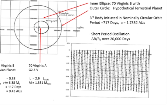
Figure 14. Layout of 70 Virginis A and B system with B in elliptical path interior to HZ planet 1.7 AU. Shown as in initially circular orbit, HZ planet experiences short and long term ?R/R₀ variations.

Clearly, with increasing mass of 70 Virginis B, the stability of a terrestrial planet in the HZ will suffer. Our nominal case indicates effective “extremities” cycling over 3400 years to +0.22 and -0.3 (Figure 15). The more likely middle value (45 degree inclination) increases the mass from around 6 Jupiters to ~9, the cycle length reduces to 2500 years and the minimal distances to A become lower, as can be inferred from the 75° inclination results of -0.4. I suspect we narrowly missed “The End” here.

We have not spent much space dwelling on thermal effects of cycles of ?R/R₀, but Figure 15 maps the first order effect for the 70 Virginis planetary system aligned with the line of sight (M_B = 6.38 Jovian masses). About 1700 terrestrial years into the cycle, the stellar effective temperature (at the surface surrounding the heat source at a given radial distance) varies.

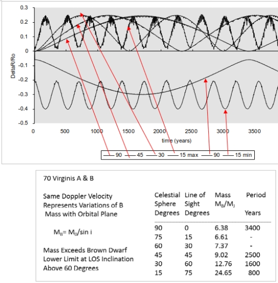
Figure 15. Oscillations of HZ planet due to 70 Virginis B mass. Mass lower limit based on observing B object in plane perpendicular to celestial sphere.

As stated earlier, thermal equilibrium conditions on a terrestrial planet are complicated due to several factors, but considering a half-lit sphere with a given albedo or reflectance, we can set planetary body at equilibrium near the freezing point of water in a circular orbit representing a temperate environment. But then when it is shifted over thousands of years into an eccentric orbit in which equilibrium temperatures could increase tens of degrees above during summer and sink below in winter seasons, we can see how they could get quite harsh during the most eccentric phases. It should be noted that these are increases in annual extremes, but due to elliptical motion, the cumulative effect of the new heating rates probably needs further consideration to determine whether they imply eras of ice or hot drought.

In the case of the HZ planet in orbit about Alpha Centauri A, we observed an 8000 year eccentricity cycle with an amplitude of about +/- 0.09 of initial radius. OK, but one could well ask, “Why?” What’s responsible? Rather than examining the RE3BP at length, we provide here an indication of what happens when we vary the eccentricity of Alpha Centaur A and B, keeping their same mean distance of separation and their masses.

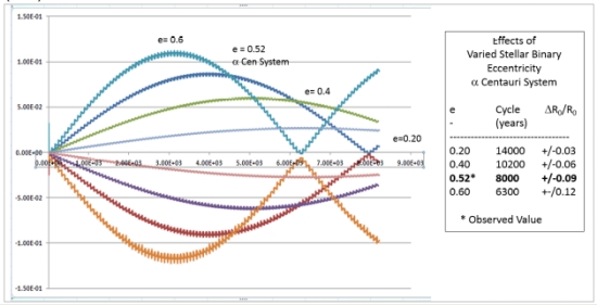
Figure 16. Varying Alpha Centauri binary system eccentricity – effect on HZ planet orbit about A.

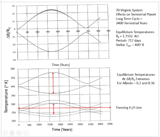
Figure 17. ?R/R₀ max and min variations over thousands of years results in HZ planet experiencing variations in winter and summer season intensities based on radial distances.

In Figure 17 the 70 Virginis case tipped the effective stellar temperature about 70 degrees higher at HZ planet summer with a corresponding drop by 45 degrees in winter due to radial distance. The Earth’s radial variations do not impose much temperature difference in the current era in comparison with the axial tilt and exposure of southern and northern hemispheres. At this point, with a hypothetical planet, we have no idea what its rotation might be, nor its tilt to the local plane of the ecliptic. But binary system dynamics indicate powerful forces driving climate conditions.

For 47 Ursae Majoris, my suspicion is that the best solution for a habitable world would be life as a satellite orbiting it and that this massive Jupiter’s internal energy will make up the balance for the heat it needed. But it would still be a novel situation with the system’s angular accelerations in the 47 Ursae Majoris binary. But the alternative scenario of establishing a circular orbit in midst of the HZ, as shown in Figure 18, provides faint hope of stability over thousands of years.

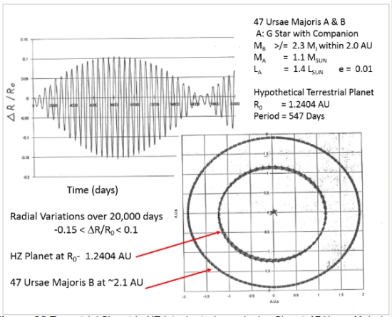
Figure 18. Terrestrial planet in HZ interior to large Jovian planet 47 Ursae Majoris B.

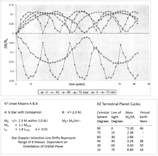
Figure 19. Mass variations of B influence on HZ planet with orbital plane inclination

As you can see from our initial discussion, in the mid-1980s it was not clear that there would ever be any exoplanets to consider, whether from theory, the result of detection or at the particular set of stars systems selected. It was one thing to place a planet in an HZ orbiting a star completely similar to the sun, another to place it where the star (or stars) were not similar, and still another thing to consider the dynamical effects of binary systems. You might see a dual star-set or star-rise in a Star Wars movie, but it might not be any more real than the flight of an ostrich even though it has all the necessary feathers. All I knew at this point was that two binary stars could revolve around their center of mass and influence a minor body in a manner known to mechanics as the Restricted 3-Body Problem. For the infinitesimal third body, it might be stable, or it might not – and it might take a long period of observation to make a useful assessment. After all, even with the Earth in the solar system there are limitations to its warranty.

Historically, what has driven much of Three Body Problem study has been the Earth, Moon and Sun system – of concern to 18th century mathematicians such as Lagrange, and then the system created by the Earth, Moon and a spacecraft. The latter fostered American research on behalf of NASA for lunar exploration by Victor Szebehely and others. Professor Szebehely’s 1960s text Theory of Orbits is, of course, a classic.

The two systems of principal interest in the Solar System, beside having very small third bodies, had something else in common. They both had low eccentricities. If you hadn’t noticed it before the discovery of numerous exoplanets, stellar binaries frequently have high eccentricities like asteroids and even comets. The Alpha Centauri system binary eccentricity is about 0.52; the two stars spring and fall back within the bounds of the system over a near 80 year period. They don’t careen into each other’s habitable regions, but their gravitational influence and their changing angular velocities about their common center of mass are both considerations of concern. Simulation would be characterization and then there would be plenty of consequences of results to consider.

Nonetheless there were some pioneer studies. Your best bet was find a large library and look for articles and cross references. David Black, for example, at NASA Ames had done some simulations of binary star system planets in the late 70s. And it was my luck that he was Director of the Lunar and Planetary Science Institute when I moved to Houston in 1986. He was editor and a contributor to an early publication about exoplanet search (TOPS – Toward Other Planetary Systems) which surveyed the 1980s era accomplishments thus far and the instruments that could be applied to the search in the future. It was near enough a Bible for the time. When I moved back to Houston to work, the Lunar and Planetary Science Institute, established for the Apollo missions, was in my neighborhood, its conferences accessible, and there were opportunities to talk directly with Dr. Black. In fact, at least one of those “conferences” was in seats in the same row of a flight home, each of us returning from business trips.

Elsewhere, at Stony Brook, the State University of New York (SUNY) in 1996, rather than a majority of geophysicists and geologists, there was a crowd of well-known observers and stellar formation theorists who were now venturing into the study of exoplanets. Many of the invited participants are still active today. Indeed, some had made the trail-blazing exoplanet. brown dwarf and CSD discoveries! Since the title of the conference addressed planets in binary stars, how could I have ignored the opportunity to participate?

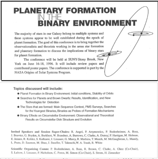
I wish I could give a full survey of the papers and discussions in 1996 and describe how much excellent work in parallel was going on. It would be better to read the papers and presentations directly. At the very least, I should note that in parallel, Matthew Holman and colleagues at the University of Toronto were examining Alpha Centauri HZ dynamic stability with a wide range of inclinations with respect to the binary plane. There were numerous talks on migrating planets, CSDs and detections of planetary candidates. But to give an indication of how tentative those earlier days were, when was the last time you heard a discussion about the viability of Bode’s Law? Yet despite only a small set of large, hot planets, more and more analysts had increased faith in circumstellar disks (CSDs) producing planets within their ten million year lifetimes. The belief rested on evidence arriving through the widening and more sensitive spectral window, both ultraviolet and infrared, thanks to satellite observatories ROSAT and IRAS. Photometric excesses beyond the usual near black body stellar spectral profile both on the UV and IR edges of T Tauri stellar spectra were mapped and analyzed to indicate massive clouds of gas and dust which could potentially be forming into planets. The hot Jupiters detected early on looked suspiciously like they had coasted into the regions near their parent stars.

Ideas were exchanged about how gas giant planets could wander. Essentially, when one small spacecraft’s path is deflected by passage by Jupiter or Saturn (e.g., Voyager), there is an exchange of momentum. The spacecraft is deflected off into space and Jupiter or Saturn is kicked infinitesimally in the other direction. In the early days of star system formation, the clouds of dust and gas constitute many magnitudes more exchange if the disk contains matter enough to form planets, enough to allow the newly formed giants to slip close to their star. This was evidenced by discoveries of Mayor, Queloz, Marcy and Butler. But would migration end generally with gas giants actually consumed by their suns? Were some ejected? Or could they end up like Jupiter and Saturn? All very tentative as well. While this was positive evidence of planets, it also made many wonder whether most planets drifted even closer to their suns and vanished. In other words, Earth’s odds for existence what with Jupiters migrating, maybe stampeding headlong toward their parent stars… That left our odds for Earth’s repetition as low.

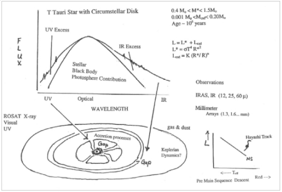
Figure 20. Circumstellar disk provides photometric excesses in UV and IR surrounding T-Tauri Stars. Detected by orbital observatories ROSAT and IRAS respectively.

The American Astronautical Society, the aerospace professional organization most concerned with celestial mechanics or astrodynamics, tends to hold its conferences at ski lodges during the summer. I presented results with them several times, the last time in 1997 at Sun Valley, Idaho. Many of the plots in this report are drawn from that report. To those curious about exoplanet existence, it might come as a surprise that most questions or comments concerned better methods for tracking their destruction, their failure modes, as it were, with better regulated time steps or integration algorithms. The remarks were right, of course, but if these planets were falling off their existential tightropes due to 3rd body interactions, why not just close their cases?

It should also be noted, that the stability tables for Alpha Centauri A and B indicate that the HZ around B provides less eccentricity variation at that 400 degree Kelvin reference point. It is fair to say that things look more stable for life at the B star than the A, though the HZ is not built to the same large scale.

Assuming that our descendants can somehow solve the problem of getting to Alpha Centauri A and B, I doubt that transfer difficulties between each star’s putative HZ exoplanets will deter visits. But the difficulties are worth noting, considering what our present-day infrastructure allows us to do in the Solar System. We tend to employ minimum energy paths between paths involving 180 degree passages, the Hohmann transfer. Were we to do so between these two stars, the transit would take decades. Moreover, if readers are familiar with setting up transformations between fixed and rotating coordinate systems, they probably share sighs of relief to observe systems that rotate at constant rates. Highly elliptic binaries are exceptions to such clockwork. If you want to establish an initially circular orbit around a star, it might even be faster to try trial and error than to calculate circular orbit based on all the terms, especially at off X axis points. Then, if you are headed away from a planet in Alpha Centauri A HZ to a planet in the B HZ, you will need excess of planetary escape velocity to set you off on a star B capture path. Certain elliptic paths will get a spacecraft captured by the other star, but then you have to contend with both planetary and stellar positons and velocities.

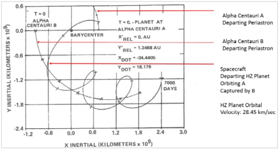
Figure 21. A spacecraft launches from HZ of Alpha Centauri A for capture into the system of B

In Figure 21, in which the inertial velocities of a transfer velocity are provided from a start near the periastron passage of the two stars A and B, with A revolving counterclockwise about the barycenter and B counter-clockwise as well on a wider ellipse. At A the local circular HZ planetary orbital velocity is about 28.74 km/sec, a little slower than the Earth’s orbital rate around the sun. The HZ orbital radius is about 25% wider than the sun’s owing to greater Alpha Centauri A brightness and the stellar mass is assumed slightly greater as well. As indicated in the figure, in the inertial coordinate system of the binary star motions, the escape and capture velocity of a spaceship exiting the HZ of A was 34.44 km/sec in the minus X direction and 18.179 in the positive Y direction, a velocity magnitude of 38.944 km/sec. The planet was located directly above the periastron-apoastron axis of the binary, indicating that the maneuver exploited both the x axis rotational velocity of HZ planet and the periastron velocity of the Alpha Centauri A, shall we say, to conserve propellant. To first order, an impulsive rocket maneuver (discounting escape from the HZ planet’s gravitational field), provided 5.7 km/sec in negative x direction and 12.5 km/sec in y axis (assuming Alpha Cen A at periastron is ascending at 5.789 km/sec in the inertial frame). This gives 13.73 km/sec change in velocity for a maneuver to jump from one binary component to another.

Here, Figure 22 is an update on the trajectory plotted in Fig. 21 three decades ago. It turns out that the trajectory is a “cycler” between the two binary stars. It orbits each for two stellar revolutions and then is ejected after 300 years.

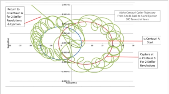
Figure 22. Departure from Alpha Centauri A HZ orbit to B.

Clearly our stellar navigation task is still far from done. We will need to aim in the B system to intercept the HZ planet in some phase of its orbit. There is a similar HZ target at about 0.65 AU radius about B. The orbit might be elliptic and it might NOT be in the same plane as we have been working so far. In fact, there is no guarantee that either star system’s planets will share the same plane of orientation as the binary stars.

Planets Leaping Orbits like Electrons?

Regarding binary system planets with semi-axes of the same values but different eccentricities, if the eccentricity exceeds that of cycle such as we have described, there can be established a whole other cycle of oscillations over thousands of years enveloping the less extreme cycle (Figure 13). Often enough I have seen stability diagrams where contour lines are shown, but I am surprised to see them appearing as natural orbital zones, save in quantum mechanics, e.g., electron angular momentum quantum numbers in the hydrogen atom. What would cause a planet to jump? Probably the influence of another large planet in the star system. And unless a stable resonance is established, the two planets could eventually collide.

Initial velocities required radial as well as tangential components with respect to MA. For our nominally circular orbit case at T_EFF = 400° K, eccentricity varies between near zero and about 0.09 over an 8,000 terrestrial-year cycle. Figure 23 shows results for three initial e_I values: 0.04, 0.09 and 0.15. These three values are respectively within, at the edge and well beyond the eccentricity bounds of the initially circular case (e_I = e_o = 0.). In Fig. 23, all three cases are 90 – 100° out of phase with the base case, but the lowest e_o case did in fact return to near zero value. Some overlap appears in ?R/R_o values for 0.04 and 0.09 cases, but the 0.15 case does not flatten out to values below the 0.09 case peak. Some remaining dynamic effects prevent the two low e_I orbits from coinciding, but in gross terms they are much the same. Allowing for variation in initial true anomaly, the three cycles appear nearly of equal duration, but phase shifts over tens or hundreds of thousands of years could result in eccentricity intersections. While I doubt that there would be two or more terrestrial planets in the HZ, these oscillations might be significant in the planetary formation process starting with smaller bodies. Additionally, after a terrestrial planet is formed, some fourth body interaction could perhaps cause a planet to jump from one state to another. Imagine Jupiter and Saturn being more massive, and perhaps the Earth or Mars would reach such thresholds. If we describe such behavior of electrons near nuclei, the Bohr Atom, can we speak of the Bohr star system?

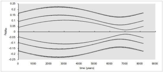
Figure 23. Centauri A planet with fixed a_pl, varied initial eccentricity. Demonstration of angular momentum bands R_o = a_pl = 1.2468 AU, e_I = .04,.09, .15

Back from the Stars and to the Moon

Nearly a decade after the Sun Valley Astrodynamics conference report, I found myself involved in some of the preparatory work for sending astronauts back to the moon. In the group I was working with, there were questions arising about Earth-Moon trajectories, Lagrangian points and stable 3rd body orbits which I needed to work on. The patched conic two body calculations that I had learned or used in college to follow the Apollo program were not adequate for the occasion. But if you look at a stellar binary system like a red dwarf and gas giant as large or larger than Jupiter with low eccentricity, you have a very close cousin to the Earth-Moon system in dynamic behavior… Again I started cutting and pasting code and I was back in the solar system, examining crew exploration trajectories back and forth between Earth and Moon (Figure 24).

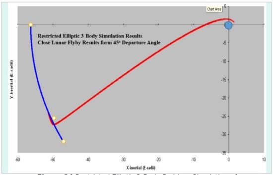
Figure 24. Restricted elliptic 3-Body Problem simulation of spacecraft launched to orbit the Moon.