Centauri Dreams
Imagining and Planning Interstellar Exploration
A New Search Space for Exomoons?
Given our recent discussion of exomoon candidate Kepler-1708 b-i, a possible moon 2.6 times the mass of Earth orbiting a gas giant, I want to be sure to work in Miki Nakajima’s work on how moons form. Nakajima (University of Rochester) is first author of the paper describing this work. It’s a significant contribution because it points to a way to refine the target list for exomoon searches, one that may help us better understand where to look as we begin to flesh out a catalog of these objects..
And flesh it out we will, as the precedent of the rapidly growing exoplanet count makes clear. What I want to do today is consider how we’ve thus far proceeded. You’ll recall that when David Kipping and team performed their deep analysis of the data leading to Kepler-1708 b-i, they chose gas giants on orbits with a period of 400 days or more, so-called ‘cool worlds’ more like Jupiter than the ‘hot Jupiters’ found so frequently in early exoplanet studies. The method produced a strong candidate indeed.
But Nakajima’s work suggests that when it comes to fractionally large moons, super-Earths should be high on the target list. We need as large a moon as possible, one having the maximum gravitational effect on its planet so that it produces the most observable signature in terms of transit timing variations of the host world around its star. Working with colleagues at Tokyo Institute of Technology and the University of Arizona, Nakajima has concluded that rocky planets larger than 6 Earth masses are unlikely to produce large moons, as are icy planets larger than a single Earth mass.
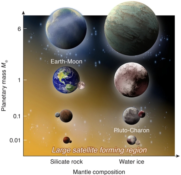
Image: This is Figure 6 from the paper, titled “Schematic view of the mass range in which a fractionally large exomoon can form by an impact.” Caption: The horizontal axis represents the mantle composition and the vertical axis represents the planetary mass normalized by the Earth mass M?. Rocky planets smaller than 6?M? and icy planets smaller than 1?M? are capable of forming fractionally large moons as indicated by the orange shading. Our prediction is consistent with planet–moon systems in the solar system. Credit: Nakajima et al.
These conclusions grow out of computer simulations, modeling the kind of impact scientists generally believe produced our own fractionally large moon. In this view, the so-called Theia impactor, an object perhaps the size of Mars, struck the Earth early in its development, creating a partially vaporized disk around the planet that eventually produced the Moon. Nakajima’s team ran simulated rocky planets as well as icy worlds through collision scenarios, varying their masses and examining the resulting disks.
As to the parameters of the simulation, note this:
In this work, we use the fixed impact angle (??=?48.6°) and the impact velocity (vimp?=?vesc), where vesc is the mutual escape velocity. The impact angle and velocity are similar to those for the canonical moon-forming impact models. The reason why we explore different mass ranges for the rocky and icy planets is that the required mass for complete vaporization is different between them…
The key to the results is the nature of the debris disk. A partially vaporized disk, like the one that presumably produced our own Moon, cools in these simulations and allows accreting ‘moonlets’ to emerge. These will eventually aggregate into a moon. But when the collisional disk is fully vaporized, these constituent parts experience strong drag from the vapor, causing them to disperse and fall onto the planet before forming a moon.
The six Earth mass cutoff marks the point in these simulations at which these planetary collisions begin to produce fully vaporized disks, rendering them incapable of forming the kind of fractionally large moons that will be easiest to detect. This finding could shake things up, because thus far we have been examining a search space largely defined by gas giants. From the paper:
Our model predicts that the moon-forming disk needs to be initially liquid or solid rich, supporting the canonical moon-forming impact model. Moreover, this work will help narrow down planetary candidates that may host exomoons; we predict that planets whose radii are smaller than ~1.6R? would be good candidates to host fractionally large exomoons (?6 M? for rocky planets and ?1 M? for icy planets). These relatively small exoplanets are understudied (only four out of 57 exoplanets surveyed by the HEK [Hunt for Exomoons with Kepler] project are under this radius limit), which can potentially explain the lack of exomoon detection to date.
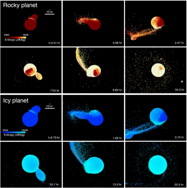
Image: This is Figure 1 from the paper, titled ‘Snapshots of giant impacts.’ Caption: The top two rows represent an impact between two rocky planets. The red-orange colors represent the entropy of the mantle material (forsterite). The iron core is shown in gray. The bottom two rows represent an impact between two icy planets. The blue-sky-blue colors represent the entropy of water ice, and the orange color represents forsterite. The scale represents 107?m. Credit: Nakajima et al.
Refining our target list is crucial for maximizing the return on telescope time using our various space-based assets, including the soon to be functioning James Webb Space Telescope. The paper continues:
Super-Earths are likely better candidates than mini-Neptunes to host exomoons due to their generally lower masses and potentially lower H/He gas contribution to the disk. This narrower parameter space may help constrain exomoon search in data from various telescopes, including Kepler, the Hubble space telescope, CHaraterising ExOPlanet Satellite (CHEOPS), and the James Webb Space Telescope (JWST).
As you would imagine, I went to David Kipping (Columbia University) for his thoughts on the Nakajima et al. result, he being the most visible exponent of exomoon research. His response:
“My main comment is that I’m pleased to see a testable theory regarding exomoons around terrestrial planets finally emerge. If scaled-up versions of the Earth-Moon system are out there up to 6 Earth masses, then we have a great shot at detecting those using HST/JWST.”
That science fictional trope of an Earth-sized moon orbiting a habitable zone gas giant may soon be joined by this new vision, large exomoons around super-Earths — even ‘double planets’ – which offer even more plot fodder for writers looking for exotic interstellar venues. Robert Forward’s Rocheworld inevitably comes to mind.
The paper is Nakajima et al., “Large planets may not form fractionally large moons,” Nature Communications 13, 568 (2022). Full text.

Planetary Birth around Dying Stars
Half a century ago, we were wondering if other stars had planets, and although we assumed so, there was always the possibility that planets were rare. Now we know that they’re all over the place. In fact, recent research out of Katholieke Universiteit Leuven in Belgium suggests that under certain circumstances, planets can form around stars that are going through their death throes, beginning the transition from red giant to white dwarf. The new work homes in on certain binary stars, and therein hangs a tale.
After a red giant star has gone through the stage of helium burning at its core, it is referred to as an asymptotic giant branch star (AGB), on a path that takes it through a period of expansion and cooling prior to its becoming a white dwarf. These expanding stars lose mass as the result of stellar wind, up to 50 to 70 percent of the total mass of the star. The result: An extended envelope of material collecting around the object that will become a planetary nebula, a glowing shell of ionized gas.
In binary systems, that stellar material coming off the star can evolve in interesting ways. While our standard view of planet formation involves circumstellar disks and planets emerging not all that long after the birth of their star, the KU Leuven work, led by Jacques Kluska, notes that in binary stars, a second star can gravitationally shape the gas and dust being ejected by a late stage red giant. From an observational perspective, this disk looks much like the disks that form around young stars.
To analyze the matter, the KU Leuven team assembled a catalog of all known post-AGB binaries that showed disks, compiling spectral energy distributions of 85 systems and examining the infrared characteristics of the various disk formations. Out of this emerged a catalog of different disk types. This is where things get intriguing. Between 8 and 12 percent of the cataloged systems are surrounded by what the paper calls ‘transition disks,’ meaning disks that show little or no low-infrared excess.
At the same time, these disks demonstrate a link with the depletion of refractory elements (metals highly resistant to heat) on the surface of the red giant star.
Jacques Kluska explains the significance of this result:
“In ten per cent of the evolved binary stars with discs we studied, we see a large cavity in the disc. This is an indication that something is floating around there that has collected all matter in the area of the cavity… In the evolved binary stars with a large cavity in the disc, we saw that heavy elements such as iron were very scarce on the surface of the dying star. This observation leads one to suspect that dust particles rich in these elements were trapped by a planet.”
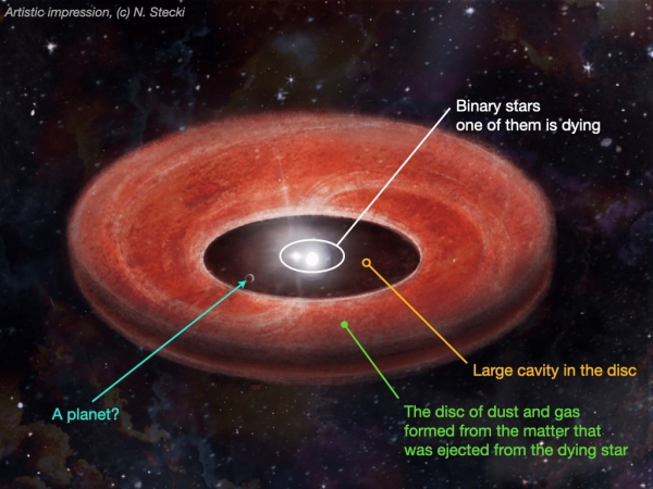
Image: Discs surrounding so-called evolved binary stars not uncommonly show signs that could point to planet formation. Credit: N. Stecki.
In this scenario, it is possible that not just single planets but an entire system’s worth could eventually grow. We’ll have to see whether planets can be confirmed in some of these systems, and to do that the team intends to home in on the ten pairs of binary stars whose disks demonstrate a large cavity. Such confirmation would denote yet another method of planet formation, to add to what we’re learning about planets in white dwarf systems. The tendency of stars to grow planets, it seems, can manifest itself even in stellar death, a useful fact given that perhaps a third of all stars in the Milky Way are found in multiple star systems. And there is precedent:
…if the planetary explanation is correct for transition disks, it would mean that there is a pressure maximum outside the planet’s orbit, trapping the dust and creating a favorable environment for second-generation planet formation… The possibility of second-generation planet formation is further supported by the detection of two giant planets around the white-dwarf binary system NN Ser. These planets are candidates for having been formed in such second-generation disks… If the planetary scenario is confirmed, these disks would become a promising site for studying second-generation planet formation and, hence, planet formation scenarios in an unprecedented parameter space.
About 1700 light years away, NN Serpentis is a system containing an eclipsing white dwarf and an M-class dwarf. The existence of what are evidently two gas giants here has been inferred from transit timing variations that can be attributed to one planet of about 6 times Jupiter’s mass, the other of about 1.6 times Jupiter’s mass, both in circumbinary orbits around this extremely tight binary. This is an interesting system for models of planet formation that go well beyond the infancy of the host stars.
The paper is Kluska et al., “A population of transition disks around evolved stars: fingerprints of planets. Catalog of disks surrounding Galactic post-AGB binaries,” Astronomy & Astrophysics Vol. 658, A36 (01 February 2021). Full text. On NN Serpentis, see Völschow et al. ”Second generation planet formation in NN?Serpentis?” Astronomy & Astrophysics Vol. 562 (February 2014) A19 (abstract). For more on late binary systems, see Winckel, “Binary post-AGB stars as tracers of stellar evolution,” in Beccari, ed., The Impact of Binary Stars on Stellar Evolution, Cambridge University Press, 2019 (preprint).
Unusual Transient: A New Kind of Magnetar?
Every time we look in a new place, which in astrophysics often means bringing new tools online, we find something unexpected. The news that an object has been detected that, for one minute in every 18, becomes one of the brightest radio sources in the sky, continues the series of surprises we’ve been racking up ever since first Galileo put eye to telescope. So what is this object, and why is it cause for such interest?
Here’s astronomer Natasha Hurley-Walker (Curtin University/International Centre for Radio Astronomy Research), who is lead author of the paper on the discovery:
“This object was appearing and disappearing over a few hours during our observations. That was completely unexpected. It was kind of spooky for an astronomer because there’s nothing known in the sky that does that. And it’s really quite close to us—about 4000 lightyears away. It’s in our galactic backyard.”
![]()
Image: A new view of the Milky Way from the Murchison Widefield Array in Western Australia, with the lowest frequencies in red, middle frequencies in green, and the highest frequencies in blue. The star icon shows the position of the mysterious repeating transient. Credit: Dr Natasha Hurley-Walker (ICRAR/Curtin) and the GLEAM Team.
Transients are nothing new to astronomers, but they usually don’t appear in this configuration. Pulsars can appear to flash on and off on cycles of milliseconds or even seconds, a fact that originally caused a flutter of SETI excitement when Jocelyn Bell (now Jocelyn Bell Burnell) and team went to work identifying their origin in November of 1967. The discovery of multiple sources of this nature soon made it clear that LGM1 (Bell’s joking reference to possible ‘little green men’) needed a less sensational name.
Slower transients are also common, the most obvious being supernovae, which can put on a celestial show before doing a slow fade that can take months. What distinguishes the new object is that it flashes on and off on a scale of minutes. It’s also emitting highly polarized radio waves, an indication that it possesses a strong magnetic field. Hurley-Walker suggests the possibility of an ‘ultra-long period magnetar,’ which would be a slowly spinning neutron star, and an unusually bright one at that.
Magnetars are neutron stars possessing a strong magnetic field. In an email exchange with Dr. Hurley-Walker, I learned that about 30 magnetars are currently known, most of them detected through X-ray observations. Most of these spin with periods between 1 and 10 seconds, and six of them have an unusual property: They flare suddenly at X-ray wavelengths and follow this with radio emission that can last for weeks, even months afterwards.
Several puzzling things leap out about the new discovery, as Hurley-Walker explained:
How is it producing radio waves, when it is spinning so slowly that it shouldn’t have enough energy? Are its magnetic fields getting twisted and it’s producing temporary emission like a radio magnetar?
How did it get to be so slow — if it aged “normally”, then its magnetic field should also be quite weak by now, in which case how is it producing radio emission?
How is it so bright, as bright as the youngest pulsars we know?

Image: An artist’s impression of what the object might look like if it’s a magnetar. Magnetars are incredibly magnetic neutron stars, some of which sometimes produce radio emission. Known magnetars rotate every few seconds, but theoretically, “ultra-long period magnetars” could rotate much more slowly. Credit: ICRAR.
The Murchison Widefield Array is unusually useful not only for studying this original find but also in looking for other objects that seem to be in the same category. Remember that the MWA is a precursor for the multinational Square Kilometre Array, which will connect radio telescopes in Western Australia and South Africa. The MWA is a low-frequency radio telescope operating between 80 and 300 MHz at the future site of the SKA, and its low frequency capabilities open up intriguing possibilities.
For when it comes to transients, we have a world of options in the high-frequency radio sky, from the above-mentioned supernovae to accretion events of various kinds, but beyond the pulsars we’ve already examined and studies of galactic nuclei, the low-frequency sky has been relatively tame. The paper on this work points out, however, that these wavelengths are sensitive to polarized radio emission processes like those at work here, fertile terrain for chasing down new transients.
This source, as an evidently slow rotator, stands out as a new category of magnetar, and one that could establish a possible population of slow-spinning magnetars that may in fact turn up in archival data at the MWA itself. Finding out whether this is the case or if we’re looking at an odd, one-off detection will take considerable digging. All of the data the MWA has produced for close to a decade is available at the Pawsey Research Supercomputing Centre in Perth, which houses MWA system data.
That’s a massive dataset, but future observations are in the cards as well. In her email, Hurley-Walker pointed to the way forward:
The MWA is currently down for maintenance but I’m planning to observe this source when it comes back up, as well as the rest of our galaxy, to try to find more of these objects. The source itself seems to be quiet at the moment, and (as far as we know) has been except in those few months in 2018.

Image: Composite image of the SKA-Low telescope in Western Australia. The image blends a real photo (on the left) of the SKA-Low prototype station AAVS2.0 which is already on-site, with an artist’s impression of the future SKA-Low stations as they will look when constructed. These dipole antennas, which will number in their hundreds of thousands, will survey the radio sky at frequencies as low as 50Mhz. Credit: ICRAR, SKAO.
An object that can convert magnetic energy to radio waves at this level stood out in the MWA observations, and we can assume that if other such objects exist, they will turn up in large numbers once the SKA comes online, offering a thousand times the sensitivity. Meanwhile, Dr. Hurley-Walker has modified her MWA search strategy to more readily spot other such transients should they occur.
The paper is Hurley-Walker et al., “A radio transient with unusually slow periodic emission,” Nature 601 (26 January 2022), 526-530. Abstract.

White Paper: Why We Should Seriously Evaluate Proposed Space Drives
Moving propulsion technology forward is tough, as witness our difficulties in upgrading the chemical rocket model for deep space flight. But as we’ve often discussed on Centauri Dreams, work continues in areas like beamed propulsion and fusion, even antimatter. Will space drives ever become a possibility? Greg Matloff, who has been surveying propulsion methods for decades, knows that breakthroughs are both disruptive and rare. But can we find ways to increase the odds of discovery? A laboratory created solely to study the physics issues space drives would invoke could make a difference. There is precedent for this, as the author of The Starflight Handbook (Wiley, 1989) and Deep Space Probes (Springer, 2nd. Ed., 2005) makes clear below.
by Greg Matloff

We live in very strange times. The possibility of imminent human contraction (even extinction) is very real. So is the possibility of imminent human expansion.
On one hand, contemporary global civilization faces existential threats from global climate change, potential economic problems caused by widespread application of artificial intelligence, the still-existing possibility of nuclear war, political instability, at many levels, an apparently endless pandemic, etc.
Image: Gregory Matloff (left) being inducted into the International Academy of Astronautics by JPL’s Ed Stone.
One the other hand, humanity seems poised for the long-predicted but oft-delayed breakout into the solar system. United States and Chinese national space programs will compete for lunar resources. Elon Musk’s SpaceX has its sights fixed on establishing human settlements on Mars. Jeff Bezos’ Blue Origin is concentrating on construction of in-space settlements of increasing population and size.
Because of the discovery of a potentially habitable planet circling Proxima Centauri and the possibility of other worlds circling in the habitable zones of Alpha Centauri A and B, one wonders how many decades it will take for an in-space settlement with a mostly closed ecology to begin planning for a change of venue from Sol to Centauri.
Consulting the literature reveals that controlled (or partially controlled) nuclear fusion and the photon sail are today’s leading contenders to propel such a venture. But the literature also reveals that travel times of 500-1,000 years are expected for human-occupied vessels propelled by fusion or radiation pressure.
Before interstellar mission planners finalize their propulsion choice, an ethical question must be addressed. In the science-fiction story “Far Centaurus”, originally published by A, E. van Vogt in 1944, the crew of a 500-year sleeper ship to the Centauri system awakens to learn that they must go through customs at the destination. During their long interstellar transit, a breakthrough had occurred leading to the development of a hyper-fast warp drive.
We simply must evaluate all breakthrough possibilities, no matter how far-fetched they seem, before planning for generation ships. The initial crews of these ships and their descendants must be confident that they will be the first humans to arrive at their destination. Otherwise it is simply not fair to dispatch them into the void.
Recently, I was a guest on Richard Hoagland’s radio show “Beyond Midnight”. Although the discussion included such topics as the James Webb Space Telescope, panpsychism, stellar engineering and ‘Oumuamua, I was particularly intrigued when the topic of space drives came up.
Richard is especially interested in possible ramifications of Bruce E. DePalma’s spinning ball experiment, which has not been investigated in depth. He later sent along a 2014 e-mail released to the public from physics Nobel Prize winner Brian D. Josephson discussing another proposed space-drive candidate, the Nassikas thruster. Professor Josephson is of the opinion that this device is well worth further study, writing this:
The Nassikas thruster apparently produced a thrust, both when immersed in its liquid nitrogen bath, and for a short period while suspended in air, until it warmed to above the superconductor critical temperature, this thrust presenting itself as an oscillating motion of the pendulum biased in a particular direction. If this displacement is due to a new kind of force, this would be an important observation; however, until better controlled experiments are performed it is not possible to exclude conventional mechanisms as the source of the thrust.
It is in this area of controlled experiments that we need to move forward. A little research on the Web revealed that there are a fair number of candidate space drives awaiting consideration. Most of these devices are untested. DARPA, NASA and a few other organizations have applied a small amount of funds in recent years to test a few of them—notably the EMdrive and the Mach Effect Thruster.
Experimental analysis of proposed space drives has not always been done on such a haphazard basis. Chapter 13 of my first co-authored book (E. Mallove and G. Matloff, The Starflight Handbook, Wiley, NY, 1989) discusses a dedicated effort to evaluate these devices. It was coordinated by engineer G. Harry Stine, retired USAF Colonel William O. Davis (who had formerly directed the USAF Office of Scientific Research) and NYU physics professor Serge Korff.
Between 1996 and 2002, NASA operated a Breakthrough Physics Program. Marc G. Millis, who coordinated that effort, has contributed here on Centauri Dreams a discussion of the many hoops a proposed space drive must jump through before it is acknowledged as a true Breakthrough [see Marc Millis: Testing Possible Spacedrives]. These ideas were further examined in the book Marc edited with Eric Davis, Frontiers of Propulsion Science, where many such concepts were subjected to serious scientific scrutiny. When I discussed all this in emails with Marc, he responded:
“The dominant problem is the “lottery ticket” mentality (a DARPA norm), where folks are more interested in supporting a low-cost long-shot, rather than systematic investigations into the relevant unknowns of physics. In the ‘lottery ticket’ approach, interest is cyclical depending if there is someone making a wild claim (usually someone the sponsor knows personally – rather than by inviting concepts from the community). With that hype, funding is secured for ‘cheap and quick’ tests that drag out ambiguously for years (no longer quick, and accumulated costs are no longer cheap). The hype and null tests damage the credibility of the topic and interest wanes until the next hot topic emerges. That is a lousy approach.
“That taint of both the null results and ‘lottery ticket’ mentality is why the physics community ignores such ambitions. I tried to attract the larger physics community by putting the emphasis on the unfinished physics, and made some headway there. When the emphasis is on credibility (and funding available), physicists will indeed pursue such topics and do so rigorously. And they will more quickly drop it again if/when the lottery ticket advocates step up again.”
Marc advocates a strategic approach, which he tried to establish as the preferred norm at NASA BPP, thus identifying the most ‘relevant’ open question in physics, and then getting reliable research done on those topics, thereafter letting these guide future inquiries. He believes that the most relevant open questions in physics deal with the source (unknown) and deeper properties of inertial frames (conjectured). Following those unknowns are the additional unfinished physics of the coupling of the fundamental forces (including neutrino properties).
In light of this pivotal period in space history and the ever-increasing contributions of private individuals and organizations, it seems reasonable to conclude that now is an excellent time to establish a well funded facility to continue the work of the Stine et al. team and the NASA Breakthrough Propulsion Physics program.
The Persistent Case for Exomoon Candidate Kepler-1708 b-i
We started finding a lot of ‘hot Jupiters’ in the early days of planet hunting simply because, although their existence was not widely predicted, they were the most likely planetary types to trigger our radial velocity detection methods. These star-hugging worlds produced a Doppler signal that readily showed the effects of planet on star, while smaller worlds, and planets farther out in their orbits, remained undetected.
David Kipping (Columbia University) uses hot Jupiters as an analogy when describing his own indefatigable work hunting exomoons. We already have one of these – Kepler-1625 b-i – but it remains problematic and unconfirmed. If this turned out to be the first in a string of exomoons, we might well expect all the early finds to be large moons simply because using transit methods, these would be the easiest to detect.
Kepler-1625 b-i is problematic because the data could be showing the effects of other planets in its system. If real, it would be a moon far larger than any in our system, a Neptune-sized object orbiting a gas giant. In any case, its data came not from Kepler but from Hubble’s Wide Field Camera 3, and with but a single transit detection. In a new paper in Nature Astronomy , Kipping describes it as an ‘intriguing hint’ and is quick to point out how far we still are from confirming it.
This ‘hint’ is intriguing, but it’s also useful in making the case that what exomoon hunters need is an extension of the search space. While the evidence for Kepler-1625 b-i turned up in transit timing variations that indicated some perturbing effect on the planet, how much more useful would such variations be if detected in a survey of gas giants focusing on long-period, cool worlds, of which there is a small but growing catalog? These planets are harder to find transiting because, being so much farther from their star, they move across its surface as seen from Earth only in cycles measured in years. That means, of course, that as time goes by, we’ll find more and more of them.
But we now have a sample of 73 cool worlds that Kipping and colleagues analyze, bringing their exomoon detection toolkit to bear. The method of their selection homes in on worlds with a radius no less than half that of Jupiter, and with either a period of more than 400 days or an equilibrium temperature less than 300 K. A final qualifier is the amount of stellar radiation received from the star. Of the initial 73 worlds, three had to be rejected because the data on them proved inadequate for assessment.
So we have 70 gas giants and a deep dive into their properties, looking for any traces of an exomoon. The team sought planets in near-circular orbits, knowing that eccentric orbits would lower the stability needed to produce a moon, also looking for at least two transits (or preferably more), where transit timing variations could be detected. The model of planet plus moon needed to stand out, with the authors insisting that it be favored over a planet-only model by a factor of no less than 10; Kipping describes this as “the canonical standard of strong evidence in model selection studies.”
Out of the initial screening criteria, 11 planets emerged and were subjected to additional tests, refitting their light curves with other models to examine the robustness of the detection. Only three planets survived these additional checks, and only one emerged with a likely exomoon candidate: KIC-8681125.01. KIC stands for Kepler Input Catalog, a designation that changes when a planet is confirmed, as this one subsequently has been. Thus our new exomoon candidate: Kepler 1708-b-i.

Image: The discovery of a second exomoon candidate hints at the possibility that exomoons may be as common as exoplanets. Just as our Solar System is packed with moons, we can expect others to be, and it seems reasonable that we would detect extremely large exomoons before any others. Image credit: Helena Valenzuela Widerström.
We know all too little about this candidate other than the persistence of the evidence for it. Indeed, in a Cool Worlds video describing the effort, Kipping gets across just how firmly his team tried to quash the exomoon hypothesis, motivated not only by the necessary rigors of investigation but also by frustration born of years of unsuccessful searching. Yet the evidence would not go away. Let me quote from the paper on this:
The Bayes factor of the planet-moon model against the planet only is 11.9, formally passing our threshold of 10 (strong evidence on the Kass and Raftery scale). Inspection of the maximum-likelihood moon fit, shown in Fig. 2, reveals that the signal is driven by an unexpected decrease in brightness on the shoulder of preceding the first planetary transit, as well as a corresponding increase in brightness preceding the egress of that same event. The time interval between these two anomalies is approximately equal to the duration of the planetary transit, which is consistent with that expected for an exomoon . The second transit shows more marginal evidence for a similar effect. The planet-moon model is able to well explain these features, indicative of an exomoon on a fairly compact orbit, to explain the close proximity of the anomalies to the main transit…
That ‘pre-transit shoulder’ shouldn’t happen, and it turns up in all the models used. It looks remarkably like the signature of an exomoon. Here’s the figure mentioned above:
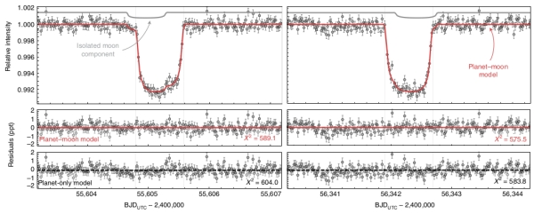
Image: This is Figure 2 from the paper. Caption: Transit light curves of Kepler-1708 b. The left/right column shows the first/second transit epoch, with the maximum-likelihood planet-moon model overlaid in solid red. The grey line above shows the contribution of the moon in isolation. Lower panels show the residuals between the planet-moon model and the data, as well as the planet-only model. BJD, barycentric Julian date; UTC, coordinated universal time. Credit: Kipping et al.
I won’t go through the complete battery of tests the team used to hammer away at the exomoon hypothesis – all the details are available in the paper – but as you would imagine, starspots were considered and ruled out, the moon model fit the data better than all alternatives, the transit signal to noise ratio was strong, and the pre-transit ‘shoulder’ is compelling. Numerous different algorithms for light curve analysis were applied to the modeling of this dataset. Indeed, the paper’s discussion of methods is itself an education in lightcurve analysis.
Describing Kepler 1708-b-i as “a candidate we cannot kill,” Kipping and team present a moon candidate that is 2.6 times larger than Earth and 12 planetary radii from its host planet, which happens to be about the distance of Europa from Jupiter. The exomoon’s mass is unknown, but constrained to be less than 37 Earth masses. The F-class host star, around which the planet orbits every 737 days, is some 5500 light years from Earth.
How such a moon might form raises a host of questions:
There are several broad scenarios for moon formation: planet-planet collisions, formation of moons within gaseous circumplanetary disks (for example the Galilean moons) or direct capture—either by tidal dissipation or pulldown during the growth of the planet. For a gaseous planet, the first scenario is unlikely to produce a debris disk massive enough to form a moon this large. The moon is also at the extreme end of the mass range produced by primordial disks in the traditional core-collapse picture of giant-planet formation, but is easier in the case where planets form by disk instability. Such models also naturally produce moons on low-inclination orbits. Direct capture by tidal dissipation is also possible, although the parameter range for capture without merger is limited. Pulldown capture can produce large moons within ~10 Jupiter radii, with a wide range of inclinations depending on the timescale for planetary growth.
In our own system, of course, we see no moons at Venus or Mercury, and it’s worth asking whether moons are rare for planets close to their host stars. Be that as it may, the supposition here is that if Neptune-sized moons do exist, they’ll constitute the bulk of our early catalog of exomoons, just as hot Jupiters dominated our early exoplanet finds. Indeed, it’s hard to see how anything smaller could be found in Kepler data.
This exomoon candidate is smaller than the previous candidate – Kepler-1625 b-i – and on a tighter orbit. While both these discoveries retain their candidate status, they hint at the possibility that large moons like these may begin turning up in JWST or PLATO data. The authors call for follow-up transit photometry for both Kepler-1708 b-i and Kepler-1625 b-i, adding “we can find no grounds to reject Kepler-1708 b-i as an exomoon candidate at this time, but urge both caution and further observations.”
The paper is Kipping et al., “An exomoon survey of 70 cool giant exoplanets and the new candidate Kepler-1708 b-i,” Nature Astronomy 13 January 2022 (full text).
A Continuum of Solar Sail Development
2020 GE is an interesting, and soon to be useful, near-Earth asteroid. Discovered in March of 2020 through the University of Arizona’s Catalina Sky Survey, 2020 GE is small, no more than 18 meters or so across, placing it in that class of asteroids below 100 meters in size that have not yet been examined up close by our spacecraft. Moreover, this NEA will, in September of 2023, obligingly make a close approach to the Earth, allowing scientists to get that detailed look through a mission called NEA Scout.
This is a mission we’ve looked at before, and I want to stay with it because of its use of a solar sail. Scheduled to be launched with the Artemis 1 test flight using the Space Launch System (SLS) rocket no earlier than March of this year, NEA Scout is constructed as a six-unit CubeSat, one that will be deployed by a dispenser attached to an adapter ring connecting the rocket with the Orion spacecraft. After separation, the craft will unfurl a sail of 86 square meters, deployed via stainless steel alloy booms. It is one of ten secondary payloads to be launched aboard the SLS on this mission.
Les Johnson is principal technology investigator for NEA Scout at Marshall Space Flight Center in Huntsville:
“The genesis of this project was a question: Can we really use a tiny spacecraft to do deep space missions and produce useful science at a low cost? This is a huge challenge. For asteroid characterization missions, there’s simply not enough room on a CubeSat for large propulsion systems and the fuel they require.”
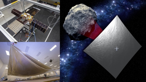
Image: NEA Scout is composed of a small, shoebox-sized CubeSat (top left) and a thin, aluminum-coated solar sail about the size of a racquetball court (bottom left). After the spacecraft launches aboard Artemis I, the sail will use sunlight to propel the CubeSat to a small asteroid (as depicted in the illustration, right). Credit: NASA.
A solar sail ought to be made to order if the objective is eventual high performance within the constraints of low mass and low volume. Reflecting solar photons and also using small cold-gas thrusters for maneuvers and orientation, NEA Scout will be investigating a near-Earth asteroid in a size range that is far more common than the larger NEAs we’ve thus far studied. It’s worth remembering that the Chelyabinsk impactor was about 20 meters in diameter, and in the same class as 2020 GE.
The 2023 close approach to Earth will occur at a time when NEA Scout will have used a gravitational assist from the Moon to alter its trajectory to approach the asteroid. Julie Castillo-Rogez, the mission’s principal science investigator at JPL, says that the spacecraft will achieve a slow flyby with relative speed of less than 30 meters per second. Using a camera with a resolution of 10 centimeters per pixel, scientists should be able to learn much about the object’s composition – a clump of boulders and dust (think Bennu, as investigated by OSIRIS-REx), or a solid object more like a boulder?
Bear in mind that NEA Scout fits into a continuum of solar sail development, with NASA’s Advanced Composite Solar Sail System (ACS3) the next to launch, demonstrating new, lightweight boom deployment techniques from a CubeSat. The unfurled square sail will be approximately 9 meters per side. As we haven’t looked at this one before, let me add this, from a NASA fact sheet:
The ACS3’s sails are supported and connected to the spacecraft by booms, which function much like a sailboat’s boom that connects to its mast and keeps the sail taut. The composite booms are made from a polymer material that is flexible and reinforced with carbon fiber. This composite material can be rolled for compact stowage, but remains strong and lightweight when unrolled. It is also very stiff and resistant to bending and warping due to changes in temperature. Solar sails can operate indefinitely, limited only by the space environment durability of the solar sail materials and spacecraft electronic systems. The ACS3 technology demonstration will also test an innovative tape-spool boom extraction system designed to minimize jamming of the coiled booms during deployment.
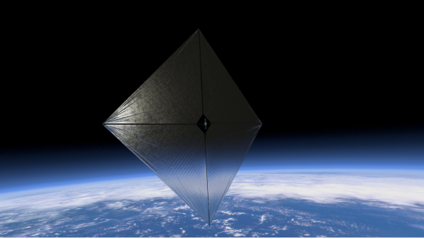
Image: An illustration of a completely unfurled solar sail measuring approximately 9 meters per side. Since solar radiation pressure is small, the solar sail must be large to efficiently generate thrust. Credit: NASA.
ACS3 is scheduled for liftoff later in 2022 as part of a rideshare mission on Rocket Lab’s Electron launch vehicle from its Launch Complex 1 in New Zealand. Beyond ACS3 looms Solar Cruiser, which takes the sail size up to 1,700 square meters in 2025, a mission we’ve looked at before and will continue to track as NASA attempts to launch the largest sail ever tested in space.

Follow with RSS or E-Mail
