Centauri Dreams
Imagining and Planning Interstellar Exploration
Laser Thermal Propulsion for Rapid Transit to Mars: Part 2
In Part 2 of Andrew Higgins’ discussion of laser-thermal rocketry and fast missions to Mars, we look more deeply at the design and consider its potential for other high delta-V missions. Are we looking at a concept that could help us build the needed infrastructure to one day support expansion beyond the Solar System?
by Andrew Higgins
We now turn to the detailed design our team at McGill University came up with for a laser-thermal mission capable of reaching Mars in 45 days. Our team took the transit time and payload requirement (1 ton) from a NASA announcement of opportunity that appeared in 2018 that was seeking “Revolutionary Propulsion for Rapid Deep Space Transit”. Although being in Canada made us ineligible to apply to this program, we adopted this mission targeted by the NASA announcement for our design study; being in Canada also means we are used to working without funding.

Image: McGill University students responsible for the design of the laser-thermal mission to Mars.
The NASA-defined payload of 1 ton would be a technology demonstration mission (what we call Mission Mars 1 in our study). Placing a premium on minimizing the transit time presumably reflects NASA’s eventual interest in lessening astronaut exposure to galactic cosmic rays, which increases sharply once a spacecraft leaves the Earth’s protective magnetosphere. Once on the surface of Mars, data from the Curiosity rover have shown that the radiation environment there appears to be more benign, comparable to or even less than the radiation exposure encountered on the ISS. Throwing regolith to cover the habitat on Mars would lower the radiation risk further, so astronauts leading a hobbit-like existence on Mars should stay healthy, provided they get there quickly.
Our Mars 1 mission starts with our spacecraft already in medium Earth orbit (MEO), so that it remains in view of the ground-based laser during the entire laser-powered burn, which takes about an hour. Given the ongoing revolution in space access, we did not bother to explore using laser propulsion to get to orbit. Chemical propulsion is well-suited for reaching orbit, so we selected a Falcon 9 to bring our vehicle to MEO and focused on using the laser for the transit to Mars.
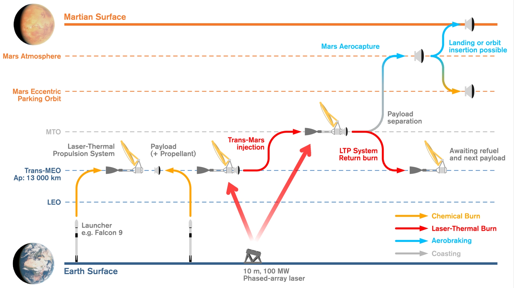
Image (click to enlarge): The concept of operations for a rapid transit to Mars mission using laser-thermal propulsion. Note the use of a burn-back maneuver to bring the laser-thermal stage back to medium Earth orbit after sending the payload to Mars.
The laser array on Earth is about 10 m by 10 m, comparable to a volleyball court, and for the 1 ton payload mission, the laser would operate at 100 MW output for an hour, using power taken from the grid or generated via solar and then stored in a battery farm. (It is worth noting that a battery farm capable of providing 100 MW for an hour was built in South Australia in 2017 from scratch in just 60 days, in response to a taunt posted in a tweet [1]. So, powering the laser is not a problem.
When the laser beam arrives at the spacecraft, it is focused into the propellant heating chamber by a large, inflatable reflector—a balloon that is transparent on one half and reflective on the other. Inflatable space structures like this are fairly mature, including a demonstration of an inflatable antenna that flew on the Space Shuttle in 1996; a comprehensive overview of this technology was given by Jamey Jacob at the 6th TVIW in Wichita [2]. Inflatable collectors such as these have shown sufficient optical quality for our purposes. While the laser flux on the inflatable is intense, we found fluorinated polyimide films have sufficiently low absorptivity to avoid overheating.
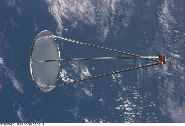
Image: Inflatable Antenna Experiment deployed from the Space Shuttle Endeavor (STS-77).
Image Source: https://apod.nasa.gov/apod/ap960525.html
The inflatable reflector focuses the laser into the heating chamber, raising the temperature of the hydrogen flowing through the chamber to greater than 10,000 K. Keeping the walls of the chamber cool is the central challenge of the design, but our team found a combination of regenerative cooling (cool hydrogen flowing through the walls), transpiration cooling (injecting hydrogen through porous walls), and seeding the hydrogen (to trap thermal radiation in the propellant, similar to the greenhouse effect) should be sufficient to keep the walls cool. The heat absorbed via regeneration is used to power the turbopumps needed to pump the hydrogen via an expander cycle. The fully ionized hydrogen propellant is then exhausted through a conventional bell nozzle to generate thrust. Based on our own calculations and prior work on laser thermal propulsion and gas-core NTRs from the 1970s, a specific impulse of 3000 s appears feasible.
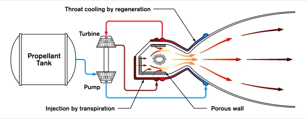
Image: Details of the propellant heating chamber and associated propellant feed and cooling systems.
The laser propulsion hardware is just dead mass once the spacecraft exceeds the focal length of the laser (which is about 50,000 km), so our team proposed bringing the laser thermal propulsion stage back to Earth via a flip-and-burn-back maneuver while still within range of the laser in cis-Lunar space. Once the propulsion stage is brough back to low or medium Earth orbit, it can be refilled and readied for use again. This would allow a single laser-thermal stage to throw multiple payloads to Mars over the duration of a given launch window.
The 14 km/s Delta-V laser thermal burn sends the spacecraft to Mars on a nearly straight line trajectory: no need for looping ellipses and Venus flybys. Our astrodynamicist optimized the trajectory for a 2020 departure. Even though our design had the launch two months after Perseverance, the vehicle would arrive at Mars three months before the newest Mars rover, overtaking it on the way.
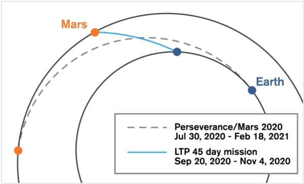
Image: 45-day transfer orbit to Mars via laser thermal propulsion, in comparison to the 7-month journey of the Perseverance rover.
When the spacecraft arrives at Mars, there is no laser to perform a laser-assisted deceleration burn (at least, not yet) and at the high approach velocity, aerocapture appears the best option. At an approach speed of 16 km/s, aerocapture is going to be harsh and is another critical link in the mission design. The heat flux will be intense, but the new Heatshield for Extreme Entry Environment Technology (HEEET) developed by NASA in recent years appears to be rated to withstand even greater heat flux. The vehicle entering the Martian atmosphere would need to use lift pointed down (toward the surface of Mars) to keep the vehicle in a trajectory that skims the atmosphere. This maneuver is a delicate balance between heat load, the g-load, and the lift and ballistic coefficients of the spacecraft, which we first modelled analytically and then backed-up with full three-degree-of-freedom simulations. The g-load limit was set at 8-gees for our study; for the scaled-up design with astronauts, the g-load will be severe and sustained for several minutes, but within the limits of what humans can tolerate. (Relevant to note that, at the recent Interstellar Symposium in Tucson, Esther Dyson reported from her centrifuge training at Star City that, “8-gees going through you was actually a lot of fun” [3]). The aerocapture would be a wild ride, for sure.
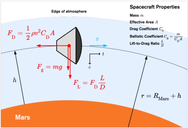
Image: Details of model used for aerocapture upon arrival at Mars.
The scaled-up version of our design (Mission Mars 2a) intended for crewed missions used a 40-ton spacecraft derived from the Orion capsule and European Service Module. The greater payload requires a more powerful (4 GW) laser to effectuate the same 45-day transit to Mars, but the laser array occupies the same 10-m footprint on earth.
The other mission we considered was a cargo mission (Mission Mars 2b). Robert Zubrin often makes the point that—even if advanced propulsion capable of high thrust and high specific impulse was available—he would still opt for a 6-month free-return trajectory and use the enhanced propulsion capability to bring more payload. So, the Mars 2b mission uses the performance of laser thermal propulsion to maximize the amount of cargo that could be brought to Mars with a Hohmann-like transfer, and shows that the payload could be increased by a factor of more than 10 over what a Centaur upper stage—with the same mass of propellant—could throw to Mars.
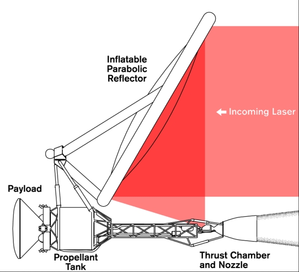
Image: Final design of laser-thermal propulsion spacecraft capable of reaching Mars in 45 days.
While a more thorough vetting of our design is called for and much work remains to be done, one encouraging finding is that the specific power of the laser thermal propulsion design is so good—an “alpha” on the order of 0.001 kg/kW—that even if the mass of the entire propulsion system were to increase by a factor of ten, the increased mass would not significantly affect the overall performance or payload capacity of the design. There is sufficient margin in the concept to accommodate the inevitable upward creep in mass that occurs as the design is refined.
Laser thermal propulsion may be well suited to other high Delta-V missions, such as flybys of interstellar comets, the mission to the solar gravitational focus, and a probe to the hypothetical Planet 9—if it is found. There is no reason the laser-thermal approach cannot be combined with laser electric propulsion or other techniques such as an Oberth maneuver. Perhaps it is best to think of laser thermal propulsion as a dragster that burns a lot of propellant quickly to get you up to speed, but from there, you can invoke laser electric propulsion that is well suited to the diminishing laser flux as the spacecraft exceeds the focal length of the laser. Appendix A in our paper details where we calculate the tradeoff between laser thermal and laser electric propulsion occurs. Hopefully, the laser-thermal concept can contribute to a further appreciation of directed energy as a disruptive technology for high-velocity missions in the solar system and beyond.
The complete details of our study can be found in our published paper: Duplay et al, “Design of a rapid transit to Mars mission using laser-thermal propulsion,” Acta Astronautica Volume 192 (March 2022), pp. 143-156 (abstract / preprint).
A browser-friendly version of the paper is available here: https://ar5iv.org/html/2201.00244
References
1. https://www.popularmechanics.com/science/a31350880/elon-musk-battery-farm/
2. J. D. Jacob, B. Loh, Inflatable technologies for interstellar missions, in: P. Gilster (Ed.), Proceedings of the 6th Tennessee Valley Interstellar Workshop, 2020.
3. https://www.youtube.com/watch?v=nHnUeM8RovE

Laser Thermal Propulsion for Rapid Transit to Mars: Part 1
Do the laser thermal concepts we discussed earlier this week have an interstellar future? To find out, applications closer to home will have to be tested and deployed as the technology evolves. Today we look at the work of Andrew Higgins and team at McGill University (Montreal), whose concept of a Mars mission using these methods is much in the news. Dr. Higgins is a professor of Mechanical Engineering at the university, where he teaches courses in the discipline of thermofluids. He has 30 years of experience in shock wave experimentation and modeling, with applications to advanced aerospace propulsion and fusion energy. His background includes a PhD (’96) and MS (’93) in Aeronautics and Astronautics from the University of Washington, Seattle, and a BS (’91) in Aeronautical and Astronautical Engineering from the University of Illinois in Urbana/Champaign. Today’s article is the first of two.
by Andrew Higgins

Directed energy propulsion continues to be the most plausible, near-term method by which we might send a probe to the closest stars, with the laser-driven lightsail being the Plan A for most interstellar enthusiasts. Before we use an enormous laser to send a probe to the stars, exploring the applications of directed energy propulsion within the solar system is of interest as an intermediate step.
Ironically, the pandemic that descended on the world in the spring of 2020 provided my research group at McGill University the stimulus to do just this. As we were locked out of our lab for the summer due to covid restrictions, our group decided to turn our attention to the mission design applications of the phased-array laser technology being developed by Philip Lubin’s group at UC Santa Barbara and elsewhere that has formed the basis of the Breakthrough Starshot initiative. If a 10-km-diameter laser array could push a 1-m lightsail to 30% the speed of light, what could we do in our solar system with a smaller, 10-m-diameter laser array based on Earth?
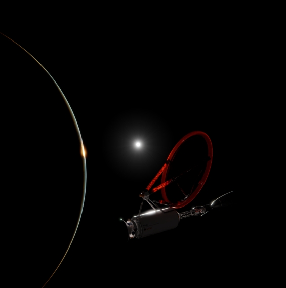
Image: Laser-thermal propulsion vehicle capable of delivering payload to the surface of Mars in 45 days.
For lower velocity missions within the solar system, coupling the laser to the spacecraft via a reaction mass (i.e., propellant) is a more efficient way to use the delivered power than reflecting it off a lightsail. Reflecting light only transfers a tiny bit of the photon’s energy to the spacecraft, but absorbing the photon’s energy and putting it into a reaction mass results in greater energy transfer.
This approach works well, at least until the spacecraft velocity greatly exceeds the exhaust velocity of the propellant; whenever using propellant, we are still under the tyranny of the rocket equation. Using laser-power to accelerate reaction mass carried onboard the spacecraft cannot get us to the stars, but for getting around the solar system, it will work just fine.
One approach to using an Earth-based laser is to employ a photovoltaic array onboard the spacecraft to convert the delivered laser power into electricity and then use it to power electric propulsion. Essentially, the idea here is to use a solar panel to power electric propulsion such as an ion engine (similar to the Deep Space 1 and Dawn spacecraft), but with the solar panel tuned to the laser wavelength for greater efficiency. This approach has been explored under a NIAC study by John Brophy at JPL [1] and by a collaboration between Lubin’s group at UCSB and Todd Sheerin and Elaine Petro at MIT [2]. The results of their studies look promising: Electric propulsion for spaceflight has always been power-constrained, so using directed energy could enable electric propulsion to achieve its full potential and realize high delta-V missions.
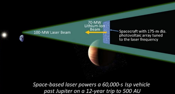
Image: Laser-electric propulsion, explored as part of a NIAC study by JPL in 2017. Image source: https://www.nasa.gov/directorates/spacetech/niac/2017_Phase_I_Phase_II/Propulsion_Architecture_for_Interstellar_Precursor_Missions/
There are some limits to laser-electric propulsion, however. Photovoltaics are temperature sensitive and are thus limited by how much laser flux you can put onto them. The Sheerin et al. study of laser-electric propulsion used a conservative limit for the flux on the photovoltaics to the equivalent of 10 “suns”. This flux, combined with the better efficiency of photovoltaics that could be optimized to the wavelength of the laser, would increase the power generated by more than an order of magnitude in comparison to solar-electric propulsion, but a phase-array laser has the potential to deliver much greater power. Also, since electric propulsion has to run for weeks in order to build up a significant velocity change, the laser array would need to be large—in order to maintain focus on the ever receding spacecraft—and likely several sites would need to be built around the world or perhaps even situated in space to provide continuous power.
I had spent my sabbatical with Philip Lubin’s group in Santa Barbara in 2018 and was fortunate to be an enthusiastic fly-on-the-wall as the laser-electric propulsion concept was being developed but—being an old-time gasdynamicist—there was not much I could contribute. There is another approach to laser-powered propulsion, however, that I thought was worth a look and suited to my group’s skill set: laser-thermal propulsion. Essentially, the laser is used to heat propellant that is expanded out of a traditional nozzle, i.e., a giant steam kettle in space. The laser flux only interacts with a mirror on board the spacecraft to focus the laser through a window and into the propellant heating chamber, and these components can withstand much greater fluxes, in principle, up to the equivalent of tens of thousands of suns. The greater power that can be delivered results in greater thrust, so a more intense propulsive maneuver can be performed nearer to Earth. The closer to Earth the propulsive burn is, the smaller the laser array needs to be in order to keep the beam focused on the spacecraft, making it more feasible as a near-term demonstration of directed energy propulsion. The challenge is that the laser fluxes are intense and do not lend themselves to benchtop testing; could we come up with a design that could feasibly handle the extreme flux?
Our effort was led by Emmanuel Duplay, our “Chief Designer,” who happens to be a gifted graphic artist and whose work graces the final design. We also had Zhuo Fan Bao on our team, who had just finished his undergraduate honors thesis at McGill on modelling the laser-induced ionization and absorption by the hydrogen propellant—the physics that was at the heart of the laser-thermal propulsion concept [3]. Heading into the lab to measure the predictions of Zhuo Fan’s thesis research was our plan for the summer of 2020, but when the pandemic dropped, we pivoted to the mission design aspects of the concept instead. Together with the rest of our team of undergraduate students—all working remotely via Zoom, Slack, Notion, and all the other tools that we learned to adopt through the summer of 2020—we dove into the detailed design.
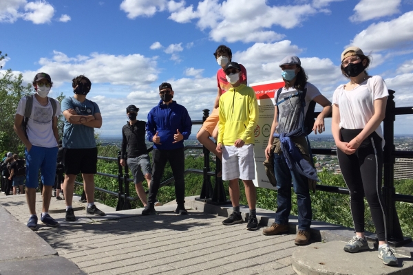
Image: McGill Interstellar Flight Experimental Research Group meeting-up in person for the first time on Mont Royal in Montreal, during the early days of the pandemic, summer 2020.
Our design team benefitted greatly from prior work on both laser-thermal propulsion and gas-core nuclear thermal rockets done in the 1970s. Laser-thermal propulsion is well-trodden ground, going back to the seminal study by Arthur Kantrowitz [4], who is my academic great grandfather of sorts. In the 1970s, the plan was to use gasdynamic lasers—imagine using an F-1 rocket engine to pump a gas laser—operating at the 10-micron wavelength of carbon dioxide. With the biggest optical elements people could conceive of at the time—a lens about a meter in diameter—combined with this longer wavelength, laser propulsion would be limited to Earth-to-space launch or low Earth orbit. To the first order, the range a laser can reach is given by the diameter of the lens times the diameter of the receiver, all divided by the wavelength of laser light. So, targeting a 10-m diameter receiver, you can only beam a CO2 laser about a thousand kilometers. The megawatt class lasers that were conceived at the time were not really up to the job of powering Earth-to-orbit launchers, which typically require gigawatts of power. For many years, Jordin Kare kept the laser-thermal space-launch concept alive by exploring how small a laser-driven launch vehicle could be made. By the 1980s, most studies focused on using laser-thermal rockets for orbit transfer from LEO, an application that requires lower power[5].
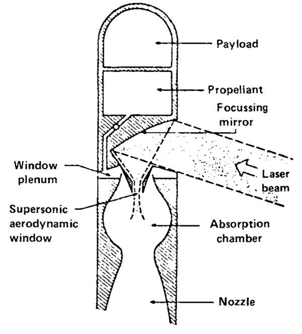
Image: Concept for a laser-thermal rocket from the early 1980s, using a 10-micron-wavelength CO2 laser. Image Source: Kemp, Physical Sciences Incorporated (1982).
As a personal footnote, I was fixated with laser-thermal propulsion in the 1980s as an undergraduate aerospace engineering student studying Kantrowitz and Kare’s work and, in 1991, visited all of the universities that had worked on laser propulsion, hoping I could do research in this field as a graduate student. I was told by the experts—politely but firmly—that the concept was dying or at least on pause; with the end of the Cold War, who was going to fund the development of the multi-megawatt lasers needed?
The recent emergence of inexpensive, fiber-optic lasers that could be combined in a phased array changed this picture and—thirty years later—I could finally come back to the concept that had been kicking around the back of my mind. The fact that fiber optic lasers operate at 1 micron (rather than 10 microns) and could be assembled as an array 10-m in effective optical diameter means they could reach a hundred times further into space than previously considered. Greater power, shorter wavelength, and bigger optical diameter might multiply together as a win-win-win combination and open up the possibility to rapid transit in the solar system.
The other prior literature we greatly benefitted from is gas-core nuclear thermal rockets. Unlike classic, solid-core NERVA rockets that are limited by the materials that make up the heating chamber, gas core nuclear thermal rockets contain the fissile material as plasma in the center of the heating chamber that does not come into contact with the walls. Work on this concept progressed in the 1960s and early 1970s, and studies concluded that containing temperatures of 50,000 K should be feasible. The literature on this topic is extensive, but Winchell Chung’s Atomic Rockets website provides a good introduction [6]. Work from the early 1970s concluded specific impulses exceeding 3000 s were achievable, but leakage of fissile material and its products from the gas core were both a performance limiting issue and an environmental nonstarter for use near Earth. But what if we could create the same conditions in the gas core using a laser, without loss of uranium or radioactive waste to worry about? The heat transfer and wall cooling issues between gas core NTR and the laser-thermal rocket neatly overlap, so we could adopt many of the strategies previously developed to contain these temperatures while keeping the walls of our heating chamber cool.
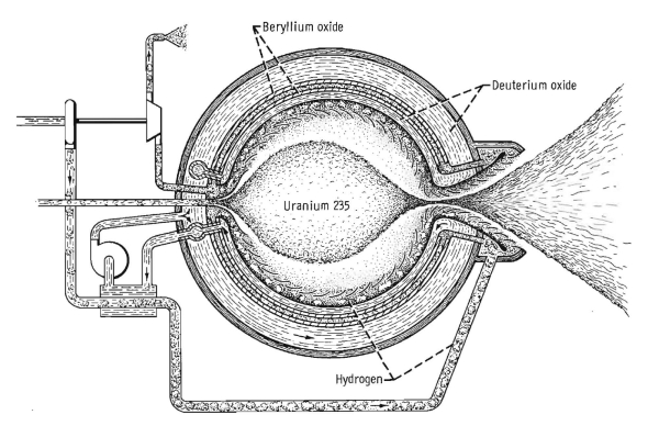
Image: Gas-core nuclear thermal rocket. Image source: Rom, Nuclear-Rocket Propulsion, (NASA, 1968).
Laser-thermal propulsion is sometimes called the poor person’s nuclear thermal rocket. Given its lack of radioactive materials and associated issues, I would argue that laser-thermal propulsion is rather the enlightened person’s nuclear rocket.
With this stage set, in the next installment, we will take a closer look at the final results of our Mars-in-45-day mission design study.
References
1. John Brophy et al., A Breakthrough Propulsion Architecture for Interstellar Precursor Missions, NIAC Final Report (2018)
https://ntrs.nasa.gov/api/citations/20180006589/downloads/20180006589.pdf
2. Sheerin, Todd F., Elaine Petro, Kelley Winters, Paulo Lozano, and Philip Lubin. “Fast Solar System transportation with electric propulsion powered by directed energy.” Acta Astronautica (2021).
https://doi.org/10.1016/j.actaastro.2020.09.016
3. Bao, Zhuo Fan and Andrew J. Higgins. “Two-Dimensional Simulation of Laser Thermal Propulsion Heating Chamber” AIAA Propulsion and Energy 2020 Forum (2020).
https://doi.org/10.2514/6.2020-3518
4. Arthur Kantrowitz, “Propulsion to Orbit by Ground-Based Lasers,” Astronautics and Aeronautics (1972).
5. Leonard H. Caveny, editor, Orbit-Raising and Maneuvering Propulsion: Research Status and Needs (AIAA, 1984).
https://doi.org/10.2514/4.865633
6. http://www.projectrho.com/public_html/rocket/enginelist2.php#gcnroc
Going Interstellar with a Laser-Powered Rocket
As far back as the 1960s, aerospace engineer John Bloomer published on the idea of using an external laser as the energy source for a rocket, using the incoming beam to fire up an onboard electrical propulsion system. And it was in a 1971 speech that Arthur Kantrowitz, looking toward the technologies that would succeed chemical rockets, suggested using lasers to heat a propellant within a rocket. This is laser-thermal propulsion, in which hydrogen (the assumed propellant) is heated to produce an exhaust stream. The hybrid method would be studied extensively in the 1970s.
So when Al Jackson and Daniel Whitmire took up the idea in a 1978 paper, they were in tune with an area that had already provoked some research interest. But Jackson and Whitmire had ideas that would refine the ramjet design introduced by Robert Bussard. They were pondering ways to power a starship, one that would carry its own reaction mass. Uneasy about the core Bussard design, the duo had, the year before, published on the idea of using a laser to augment the ramjet. Bussard sought to ignite fusion in reaction mass gathered by a magnetic ramscoop, gathering its own fuel as it roamed the galaxy. It was a dazzling idea, but problems had soon become apparent.
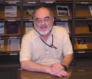
Image: Al Jackson, whose laser-powered ramjet and laser-powered interstellar rocket concepts, developed with Daniel Whitmire, refined the Bussard ramjet design and illustrated its shortcomings.
For the Bussard design, as we’ve seen not long ago in Peter Schattschneider work with Jackson (see John Ford Fishback and the Leonara Christine), runs into serious problems, including igniting the proton/proton fusion reaction Bussard advocated. We would go on to learn that the vast magnetic ramscoop of the ramjet generates far too much drag to be practical.
So Jackson and Whitmire proceeded first to come up with a laser-augmented ramjet that applied beamed energy from a transmitting installation in the Solar System, one that would interact with hydrogen collected by the starship ramscoop. They then turned their attention to beaming energy to a craft that operated using its own reaction mass rather than mass drawn from the interstellar medium.

It’s that latter idea that has the most resonance. Robert Forward in this period had been talking about beaming laser energy to space sails. Now the laser idea goes into the service of a hybrid propulsion concept that loses at least one Bussard showstopper. I’ve described Jackson and Whitmire’s idea in the past as ‘rocketry on a beam of light.’ It’s an ingenious solution, even if it does not permit us to leave the propellant behind.
Image: Daniel Whitmire, collaborator with Al Jackson on the laser-powered interstellar ramjet and rocket concepts, and author of important work on Carbon Nitrogen Oxygen cycle (CNO) fusion possibilities for the ramjet. Credit: University of Louisiana at Lafayette.
And it’s this ‘laser-powered rocket,’ as opposed to a ramjet, that should get more attention in the community than it has, given that subsequent studies of the interstellar medium have cast doubt on how even the most efficient ramscoop could collect enough reaction mass given variations in the distribution of hydrogen in the galaxy. In other words, you might have to get up to relativistic speeds in the first place just to ignite a ramjet, if indeed it could be ignited, and you would have to reckon with varying supplies of interstellar material along the way. Poul Anderson’s wonderful take on the interstellar ramjet in Tau Zero (1970) becomes highly problematic!
The laser-powered interstellar rocket contains the added advantage of being able to accelerate not only away from the laser beam but towards it, for the beam is conceived purely as an energy source, not a source of momentum. This has immediate benefits in mission planning. One of the great challenges of interstellar flight is that once you’ve managed to get your craft up to relativistic speeds, you’d like to do more upon arrival at destination than simply blitz through a planetary system at 20 percent of c. The laser-powered interstellar rocket, however, operates efficiently in both acceleration and deceleration phases. No need for Robert Forward’s ‘staged sails’ when using this take on a starship, or for the deployment of a magnetic sail as a brake.
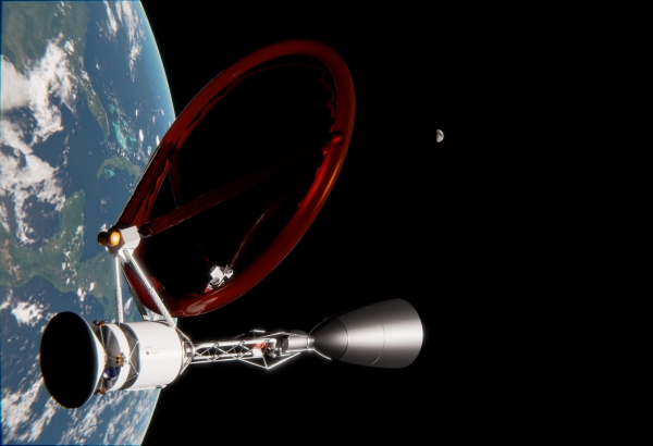
Image: Laser-thermal propelled spacecraft in Earth orbit awaiting its departure. Credit: Creative Commons Attribution 4.0 International License.
The history of interstellar studies has involved conceiving of ideas that do not break physics and then probing them to find out whether they work. Like the original Bussard ramjet and so many of Robert Forward’s ideas, Jackson and Whitmire’s concept is highly futuristic, but I love what Al said in a reminiscence on the matter in these pages: “The importance is in showing that the physics allows an opening for the engineering physics. There is no exotic physics here, only – so to speak – exotic technology.”
I sometimes forget how venerable some of these ideas are, for even while Jackson and Whitmire were doing their work on laser beaming variants to adapt the Bussard design, George Marx had already published a paper in Nature in 1966 with the provocative title “Interstellar Vehicle Propelled by Terrestrial Laser Beam.” Laser lightsails were under active discussion, and now there was a laser rocket. We have had half a century to ponder these ideas, and I see that another variant on beaming power to a spacecraft with onboard fuel has just emerged. While it’s a system advocated for fast transit to Mars, it plays upon motifs that can turn interstellar.
In a paper appearing in Acta Astronautica, lead author Emmanuel Duplay (McGill University, Montreal) and colleagues take a near-term look at what such methods can achieve. But they also give a nod to interstellar prospects, pointing out that trends like the emergence of inexpensive fiber-optic laser amplifiers and the possibility of phase-locking large arrays of such amplifiers to operate as a single element are now under active study. Moreover, adaptive optics methods can smooth beam distortions if moving through the atmosphere, allowing such an array to beam energy to a spacecraft from the surface of the Earth. Long-term, a space-based array offers huge advantages, but deep space missions do not depend on this.
Indeed, the new work responds to a recent NASA solicitation looking for propulsion concepts for rapid interplanetary missions capable of making the Earth-Mars crossing in no more than 45 days, and reaching a distance of 5 AU in no more than a year, or 40 AU (in the realm of Pluto/Charon) in no more than five years. As Mars is a feasible target for human crews in the not distant future, such a capability would mitigate the risk to astronauts of exposure to galactic cosmic rays and dangerous solar activity.
I’m intrigued by the idea that beamed propulsion can become a major factor in creating a system-wide infrastructure, one that will along the way develop the needed technologies for missions to another star. So in the next two posts, I want to turn things over to Andrew Higgins (McGill University), who is at the heart of the work in Montreal. Rapid transport to Mars is the baseline design here, but it’s a metric that not only allows us to compare competing propulsion methods but also look ahead to the deep space missions it enables.
The Jackson and Whitmire paper is “Laser Powered Interstellar Rocket,” Journal of the British Interplanetary Society, Vol. 31 (1978), pp.335-337. The Bloomer paper is “The Alpha Centauri Probe,” in Proceedings of the 17th International Astronautical Congress (Propulsion and Re-entry), Gordon and Breach. Philadelphia (1967), pp. 225-232. The paper we’ll look at next is Duplay et al, “Design of a rapid transit to Mars mission using laser-thermal propulsion,” Acta Astronautica Volume 192 (March 2022), pp. 143-156 (abstract / preprint).
A Third World at Proxima Centauri
The apparent discovery of a new planet around Proxima Centauri moves what would have been today’s post (on laser-thermal interstellar propulsion concepts) to early next week. Although not yet confirmed, the data analysis on what will be called Proxima Centauri d seems strong, in the hands of João Faria (Instituto de Astrofísica e Ciências do Espaço, Portugal) and colleagues. The work has just been published in Astronomy & Astrophysics.
It’s good to hear that Faria describes Proxima Centauri as being “within reach of further study and future exploration.” That last bit, of course, is a nod to the fact that this is the nearest star to the Sun, and while 4.2 light years is its own kind of immensity, any future interstellar probe will naturally focus either here or on Centauri A and B.
Years are short on Proxima d – the putative planet circles Proxima every five days. That’s a tenth of Mercury’s distance from the Sun, closer to the star than to the inner edge of the habitable zone. Despite some press reports, this is not a habitable zone world.
Where this work is significant isn’t simply in providing us with a third world at Proxima, but in the method of detection. When Guillem Anglada-Escudé and team found Proxima Centauri b back in 2016, they were working with data taken with the HARPS spectrograph mounted on the European Southern Observatory’s 3.6-meter telescope at La Silla. Confirming Proxima b demanded the newer ESPRESSO spectrograph, fed by the four Unit Telescopes (UTs) of the Very Large Telescope at Cerro Paranal. That work was accomplished in 2020 by researchers from the University of Geneva.
For the work on Proxima Centauri d, Faria and team used more than 100 observations of Proxima Centauri’s spectrum over two years, using ESPRESSO (Echelle SPectrograph for Rocky Exoplanets and Stable Spectroscopic Observations) to turn up the radial velocity signature of a planet in a five day orbit. The weak signal went, with further observations, from just a hint of a new world to a viable planet candidate as the team made sure they weren’t picking up an obscuring asteroseismological signal from the star itself.
The fact that Proxima Centauri d is so small – probably smaller than Earth, and no less than 26% of its mass – emphasizes the magnitude of the achievement. This is the lightest exoplanet ever measured using radial velocity techniques, surpassing the recent find at L 98-50. The planet’s RV signature demands that ESPRESSO pick up a stellar motion of no more than 40 centimeters per second. As the paper notes:
Even in the presence of stellar activity signals causing RV variations of the order of m s?1, it is now possible to detect and measure precise masses for very low-mass planets that induce RV signals of only a few tens of cm s?1.
Pedro Figueira, ESPRESSO instrument scientist at ESO in Chile, notes the significance of the find:
“This achievement is extremely important. It shows that the radial velocity technique has the potential to unveil a population of light planets, like our own, that are expected to be the most abundant in our galaxy and that can potentially host life as we know it.”
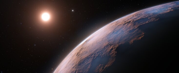
Image: A team of astronomers using the European Southern Observatory’s Very Large Telescope (ESO’s VLT) in Chile have found evidence of another planet orbiting Proxima Centauri, the closest star to our Solar System. This candidate planet is the third detected in the system and the lightest yet discovered orbiting this star. At just a quarter of Earth’s mass, the planet is also one of the lightest exoplanets ever found. Credit: ESO.
In an email this morning, Guillem Anglada-Escudé told me that Proxima Centauri d was not necessarily a surprising discovery given how many exoplanets we are now finding, but it was nonetheless ‘a very beautiful one.’ He finds the work solid:
“It is just because ESPRESSO is a new machine and Proxima has been used to benchmark it that there might be some caveats, but I find the signal strong and very convincing. Also, the only reason to be cautious here is because it is Proxima and it has scientific and cultural relevance. In summary, I would have claimed the same as the authors did. A high cadence, regularly sampled campaign should be able to confirm it with a little more effort. Unsure the ESPRESSO folks will want to invest more time on that or not.”
Anglada-Escudé went on to make another important point: The paper shows that the scientists were able to precisely measure the signal against the stellar activity background, thus separating the planetary find from the noise. The surface of the star may be marked by dark spots and convective activity. The process of ‘detrending’ cleans up the signal to eliminate spurious artifacts so that the planetary signature can be measured. Spurious Doppler shifts affect the line width and the symmetry of a signal. Detrending, said the scientist, only works well when such changes can be measured more accurately than the Doppler shifts themselves.
Thus the power of ESPRESSO. The implications for future studies are heartening:
“…this anticipates very exciting discoveries, as that should enable the detrending of RVs, especially on more sun-like stars. Whether or not ESPRESSO will be the key to solve the ‘stellar activity’ noise floor remains to be seen, but to me, it now seems to have the tools and sensitivity to achieve that.”
The paper is Faria, et al., “A Short-Period Sub-Earth Orbiting Proxima Centauri,” Astronomy & Astrophysics 658 (4 January 2022), A115 (full text).

Freeman Dyson’s Advice to a College Freshman
Anyone who ever had the pleasure of talking to Freeman Dyson knows that he was a gracious man deeply committed to helping others. My own all too few exchanges with him were on the phone or via email, but he always gave of his time no matter how busy his schedule. In the article below, Colin Warn offers an example, one I asked him for permission to publish so as to preserve these Dysonian nuggets for a wider audience. Colin is an Associate Propulsion Component Engineer at Maxar, with a Bachelor of Science in mechanical engineering from Washington State University. His research interests dip into in everything from electric spacecraft propulsion to small satellite development, machine learning and machine vision applications for microrobotics. Thus far in his young career, he has published two papers on the topics of nuclear gas core rockets and interstellar braking mechanisms in the Journal of the British Interplanetary Society. He tells me that when he’s not working on interstellar research, he can be found teaching music production classes or practicing martial arts.
by Colin Warn

Three years ago, I decided to make a switch from being a part time dance music ghost producer to study something that would help advance humanity’s knowledge of the stars. Eventually, I decided that something would be mechanical engineering, a switch which was in no small part due to space podcasts that introduced me to cool technologies such as Nuclear Pulsed Propulsion (NPP): Rockets propelled by small mini-nuclear explosions. The man behind this technology? Freeman Dyson.
Dyson worked on Project Orion for four years, deeply involved in studies that produced the world’s first and only prototype spacecraft powered by NPP. Due to the 1963 Partial Test Ban Treaty, which he supported, humanity’s best bet for interstellar travel was filed away. Yet, something about the audacity of this project resonated with me decades later when I uncovered it, especially when I found out that Dyson was in charge of this project despite not being a PhD.
So, as a bright-eyed and optimistic freshman entering his first year of college, figuring that out of anyone in the world he would have the best insights on what technology would lead humanity to the stars, I decided to send him this email:
Hello Professor Dyson,
My name is Colin Warn, and I’m a freshman pursuing a degree in mechanical engineering/physics.
Had a few questions for you regarding how I should structure my career path. My ambitions are to work on interstellar propulsion technologies, and I figured you might know a thing or two about the skill set required.
If you have the time, here’s what I’d love to hear your opinion on:
1. What research/internships would you suggest I focus on as an undergraduate to learn the skills that will be needed for working on advanced propulsion technologies? Especially in my freshman and sophomore years?
2. For my initial undergrad years, would you suggest that I focus more on taking physics or engineering courses initially?
Thank you so much in advance for your time. Been reading the book your son wrote about Orion. Let’s just say the reactions I’ve been getting from my friends when I tell them what I’m reading about is already quite fun to observe.
Regards,
-Colin

I sent it to his Princeton email, as I’ve sent many emails in the past to fairly high-caliber people, without a hope of getting anything in return.
Two days later, I woke up to find this email in my inbox.
Dear Colin Warn,
I will try to answer your two questions and then go on to more general remarks.
1. So far as I know, the only techniques for interstellar propulsion that are likely to be cost-effective are laser-propelled sails and microwave-propelled sails. Yuri Milner has put some real money into his Starshot project using a high-powered laser beam. Bob Forward many years ago proposed the Starwisp spacecraft using a microwave beam. Either way, the power of the beam has to be tens of Megawatts for a miniature instrument payload of the order of a gram, or tens of Terawatts for a human payload of the order of a ton. My conclusion, the manned mission is not feasible for the next century, the instrument mission might be feasible.
For the instrument mission, the propulsion system is the easy part, and the miniaturization of the payload is the difficult part. Therefore, you should aim to join a group working on miniaturization of instruments, optical sensors, transmitters and receivers, navigation and information handling systems. These are all the technologies that were developed to make cell-phones and surveillance drones. An interstellar mission is basically a glorified surveillance drone. You should go where the action is in the development of micro-drones. I do not know where that is. Probably a commercial business attached to a technical university.
2. For undergraduate courses, I would prefer engineering to physics. Some general background in physics is necessary, but specialized physics courses are not. More important is computer science, applied mathematics, electrical engineering and optics, chemistry of optical and electronic materials, microchip engineering. I would add some courses in molecular biology and neurology, with the possibility in mind that these sciences may be the basis for big future advances in miniaturization. We still have a lot to learn by studying how Nature does miniaturization in living cells and brains.
This email contained more detailed insights to my questions than I could have ever hoped for. Then to top it all off, he still had one more piece of advice for me to a question I hadn’t even asked.
General remarks. In my own career I never made long-range plans. I would advise you not to stick to plans. Always be prepared to grab at unexpected opportunities as they arise.Be prepared to switch fields whenever you have the chance to work with somebody who is doing exciting stuff. My daughter Esther, who is a successful venture capitalist running her own business, puts at the bottom of every E-mail her motto, “Always make new mistakes”. That is a good rule if you want to have an interesting life.
With all good wishes for you and your career, yours sincerely,
Freeman Dyson.
Upon reading this email in 2018, I promised myself that one day I’d put myself in a position to thank him in person. Sadly I’ll never get the opportunity. I discovered watching an old YouTube video featuring him that he died in February of 2020.
So this article is my way of saying thank you to him. For creating literal star-shot projects to inspire a new generation. For being someone who always questioned the status quo. But most of all, for still being down to earth enough to email some amazingly insightful answers to a freshman’s cold-email. I hope one day I’m in a position where I can pass on the favor.
An Evolutionary Path for ‘Mini-Neptunes’
It would explain a lot if two recent discoveries involving ‘mini-Neptunes’ turned out to be representative of what happens to their entire class. For Michael Zhang (Caltech) and colleagues, in two just published papers, have found that mini-Neptunes can lose gas to their parent star, possibly indicating their transformation into a ‘super-Earth.’ If such changes are common, then we have a path to get from a dense but Neptune-like world to a super-Earth, a planet roughly 1.6 times the size of the Earth and part of a category of worlds we do not see represented in our Solar System.
As we drill down toward finding smaller worlds, we’ve been finding a lot of mini-Neptunes as well as super-Earths, with the former two to four times the size of the Earth. Thus we have a bimodal gap in exoplanet observation. Where are the worlds between 1.6 and 2-4 times the size of Earth? The new work examines two mini-Neptunes around the TESS object TOI 560, located about a hundred light-years from Earth, and a pair of mini-Neptunes orbiting HD 63433, about 70 light years away. At TOI 560, the planets have periods of 6.4 days and 18.9 days; at HD 63433, the periods are 7.1 and 20.5 days.
At both stars we find a planet whose atmosphere is being stripped away, creating a large cocoon of gas. At TOI 560, it is the innermost mini-Neptune that is losing atmosphere; at HD 63433, the process is occurring on the outer world. Zhang, who is lead author of the two papers on this work, speculates that at the latter, the inner world may already have had its atmosphere stripped away; while the signature of hydrogen is found at the outer mini-Neptune, it is not detected at HD 63433 b, the inner world. The paper notes:
The predicted mass-loss timescale for planet c is longer than the age of the system, but the corresponding mass-loss timescale for planet b is significantly shorter. This implies that c could have retained a primordial H/He atmosphere, while b probably did not.
These planets are Neptune-like in having a rocky core surrounded by a thick envelope of what is thought to be hydrogen and helium. Using Hubble and Keck data for TOI 560 and HD 63433 respectively, the scientists found that at least in these systems, hot Neptunes can transform into super-Earths.
A small enough mini-Neptune close enough to its star undergoes atmospheric loss under the bombardment of stellar X-rays and ultraviolet radiation. The remnant world would be smaller in radius, while any planet in the ‘radius gap’ between 1.6 and 2-4 Earth radii would be in transition, in the process of losing much of its atmosphere over a period of hundreds of millions of years.
“Most astronomers suspected that young, small mini-Neptunes must have evaporating atmospheres,” adds Zhang. “But nobody had ever caught one in the process of doing so until now.”
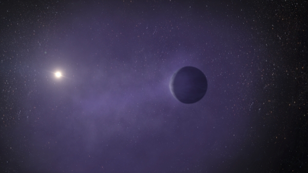
Image: This is an artist’s Illustration of the mini-Neptune TOI 560.01, located 103 light-years away in the Hydra constellation. The planet, which orbits closely to its star, is losing its puffy atmosphere and may ultimately transform into a super-Earth. Credit: Artwork: Adam Makarenko (Keck Observatory).
We have yet to determine whether the process is common, because other scenarios are possible. It is conceivable that some of the mini-Neptunes we observe are actually water worlds that are not enshrouded in hydrogen at all. As the paper on TOI 560 notes:
An alternate explanation for the radius gap is that it has nothing to do with mass loss, but is instead because cores have a broad mass distribution, with the smaller cores having never accreted gas in the first place (Lee & Connors 2021). It is also possible that some mini-Neptunes have no hydrogen-rich envelopes at all, but instead formed with substantial water-rich envelopes (e.g., Mousis et al. 2020). This could dramatically change the mass-loss rates, especially that of helium, which would have been already lost to space alongside the primordial hydrogen.
But TOI 560.01 and HD 63433 c are in the spotlight because they offer the first evidence for the theory that mini-Neptunes do become super-Earths. That evidence is strengthened by the the speed of gasses in their atmospheres. Helium at TOI 560.01 is moving as fast as 20 km/sec, while hydrogen at HD 63433 c reaches 50 km/sec.
These data are the result of transmission spectroscopy, in which light from the star is observed passing through a planetary atmosphere, thus carrying information about its composition and characteristics. The degree of motion here precludes retention by the planet, a fact that is bolstered by the size of the gas cocoons around both worlds. At TOI 560.01, the gas is detected in a radius 3.5 times that of the planet, while at HD 63433 c hydrogen is found at a distance at least twelve times the radius of the planet.
The work on TOI 560.01 involved two transits, both of which showed strong helium absorption and some evidence of variability in the atmospheric outflow. Bear in mind that this is the first mini-Neptune with a helium detection, and given that this system contains two worlds where a potential transformation into a super-Earth is possible, we have a new way to explore what Zhang calls ‘exoplanet demographics.’ From the paper:
TOI 560 is a two-planet system, and TOI 560.02 is also a transiting mini-Neptune. This makes the system an excellent test for mass-loss models. The two planets share the same contemporary X-ray/EUV environment, as well as the same irradiation history. In addition, planets of similar size located in adjacent orbits might be expected to have largely similar formation and/or migration histories, and therefore it is reasonable to expect that their primordial atmospheric compositions would be quite similar. This is supported by observational studies of the masses and radii of multi-planet systems in the Kepler sample, which suggest that planets in the same system tend to have similar masses and radii (the “peas in a pod” theory; Weiss et al. 2018).
An intriguing aspect of the situation at TOI 560 is that the innermost world shows a gas outflow that seems to be moving toward the central star. It will take future observations of other mini-Neptunes to find out just how anomalous this may be.
The papers are Zhang et al., “Detection of Ongoing Mass Loss from HD 63433c, a Young Mini-Neptune.” Astronomical Journal Vol. 163 No. 2 (17 January 2022) 68 (full text); and Zhang et al., “Escaping Helium from TOI 560.01, a Young Mini-Neptune,” Astronomical Journal Vol. 163 No. 2 (17 January 2022) 67 (full text).

Follow with RSS or E-Mail
