Centauri Dreams
Imagining and Planning Interstellar Exploration
Proxima Flare May Force Rethinking of Dust Belts
News of a major stellar flare from Proxima Centauri is interesting because flares like these are problematic for habitability. Moreover, this one may tell us something about the nature of the planetary system around this star, making us rethink previous evidence for dust belts there.
But back to the habitability question. Can red dwarf stars sustain life in a habitable zone much closer to the primary than in our own Solar System, when they are subject to such violent outbursts? What we learn in a new paper from Meredith MacGregor and Alycia Weinberger (Carnegie Institution for Science) is that the flare at its peak on March 24, 2017 was 10 times brighter than the largest flares our G-class Sun produces at similar wavelengths (1.3 mm).
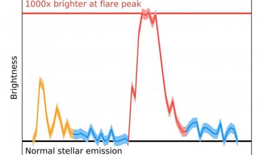
Image: The brightness of Proxima Centauri as observed by ALMA over the two minutes of the event on March 24, 2017. The massive stellar flare is shown in red, with the smaller earlier flare in orange, and the enhanced emission surrounding the flare that could mimic a disk in blue. At its peak, the flare increased Proxima Centauri’s brightness by 1,000 times. The shaded area represents uncertainty. Credit: Meredith MacGregor.
Lasting less than two minutes, the flare was preceded by a smaller flare, as shown above, revealing the interactions of accelerated electrons with Proxima Centauri’s charged plasma. We already knew that Proxima produced regular X-ray flares (recent studies have pegged the rate at one large event every few days), though these are much smaller than the flare just observed. The effects of such flaring on Proxima b could be profound, according to MacGregor:
“It’s likely that Proxima b was blasted by high energy radiation during this flare. Over the billions of years since Proxima b formed, flares like this one could have evaporated any atmosphere or ocean and sterilized the surface, suggesting that habitability may involve more than just being the right distance from the host star to have liquid water.”
The issue has significance far beyond Proxima because M-class stars are the most common in the galaxy. They’re also given to pre-main sequence periods marked by frequent changes in luminosity, and prone to a high degree of stellar activity throughout their lifetimes. Proxima Centauri, spectral class M5.5V, has long been known to be a flare star, leading to the current interest in determining the effects of its variability on the single known planet.
MacGregor and Weinberger worked with data from the ALMA 12-m array and the Atacama Compact Array (ACA). The datasets from these observations were examined by Guillem Anglada (Instituto de Astrofísica de Andalucía, Granada, Spain) in 2017, whose team found signs of a dust belt of about 1/100th of Earth’s mass in the 1-4 AU range, with the possibility of another outer belt. These two structures seemed to parallel the asteroid and Kuiper belts we find in our own Solar System, and it was thought that the inner belt might help us constrain the inclination of the Proxima Centauri system, while giving us an idea of its complexity.
I should pause to note that Guillem Anglada is not Guillem Anglada-Escudé, who led the work that discovered Proxima b — the similarity in names is striking but a coincidence. Making this even more confusing is the fact that Guillem Anglada-Escudé is a co-author on the dust paper on which Guillem Anglada was lead author. If we can get the names straight, we can go on to note that the MacGregor/Weinerger results question whether the dust belts are really there.
For MacGregor and Weinberger looked at the ALMA data as a function of observing time, noticing the transient nature of the radiation from the star. From the paper:
The quiescent emission detected by the sensitive 12-m array observations lies below the detection threshold of the ACA observations, and the only ACA detection of Proxima Centauri is during a series of small flares followed by a stronger flare of ? 1 minute duration. Due to the clear transient nature of this event, we conclude that there is no need to invoke the presence of an inner dust belt at 1 ? 4 AU. It is also likely that the slight excess above the expected photosphere observed in the 12-m observations is due to coronal heating from continual smaller flares, as is seen for AU Mic, another active M dwarf that hosts a well-resolved debris disk. If that is the case, then the need to include warm dust emission at ? 0.4 AU is removed. Although the detection of a flare does not immediately impact the claim of an outer belt at ? 30 AU, the significant number of background sources expected in the image and known high level of background cirrus suggest that caution should be used in over-interpreting this marginal result.
So we still have the possibility of an outer belt, though not one that can be claimed with any degree of certainty, and we have removed the need for the inner belt. Proxima Centauri may indeed have other planets and a more complex system than we currently know, but the data from ALMA and ACA now appear to be indicative only of the known flaring phenomenon.
“There is now no reason to think that there is a substantial amount of dust around Proxima Cen,” says Weinberger. “Nor is there any information yet that indicates the star has a rich planetary system like ours.”
The paper is MacGregor et al., “Detection of a Millimeter Flare From Proxima Centauri,” accepted at Astrophysical Journal Letters (preprint). The paper on dust belts is Anglada et al., “ALMA Discovery of Dust Belts Around Proxima Centauri,” accepted at Astrophysical Journal Letters (preprint).

Detecting Early Life on Exoplanets
At the last Tennessee Valley Interstellar Workshop, I was part of a session on biosignatures in exoplanet atmospheres that highlighted how careful we have to be before declaring we have found life. Given that, as Alex Tolley points out below, our own planet has been in its current state of oxygenation for a scant 12 percent of its existence, shouldn’t our methods include life detection in as wide a variety of atmospheres as possible? A Centauri Dreams regular, Alex addresses the question by looking at new work on chemical disequilibrium and its relation to biosignature detection. The author (with Brian McConnell) of A Design for a Reusable Water-Based Spacecraft Known as the Spacecoach (Springer, 2016), Alex is a lecturer in biology at the University of California. Just how close are we to an unambiguous biosignature detection, and on what kind of world will we find it?
by Alex Tolley

Image: Archaean or early Proterozoic Earth showing stromatolites in the foreground. Credit: Peter Sawyer / Smithsonian Institution.
The Kepler space telescope has established that exoplanets are abundant in our galaxy and that many stars have planets in their habitable zones (defined as having temperatures that potentially allow surface water). This has reinvigorated the quest to answer the age-old question “Are We Alone?”. While SETI attempts to answer that question by detecting intelligent signals, the Drake equation suggests that the emergence of intelligence is a subset of the planets where life has emerged. When we envisage such living worlds, the image that is often evoked is of a verdant paradise, with abundant plant life clothing the land and emitting oxygen to support respiring animals, much like our pre-space age visions of Venus.
Naturally, much of the search for biosignatures has focused on oxygen (O2), whose production on Earth is now primarily produced by photosynthesis. Unfortunately, O2 can also be produced abiotically via photolysis of water, and therefore alone is not a conclusive biosignature. What is needed is a mixture of gases in disequilibrium that can only be maintained by biotic and not abiotic processes. Abiotic processes, unless continually sustained, will tend towards equilibrium. For example, on Earth, if life completely disappeared today, our nitrogen-oxygen dominated atmosphere would reach equilibrium with the oxygen bound as nitrate in the ocean.
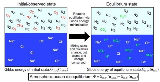
Image: Schematic of methodology for calculating atmosphere-ocean disequilibrium. We quantify the disequilibrium of the atmosphere-ocean system by calculating the difference in Gibbs energy between the initial and final states. The species in this particular example show the important reactions to produce equilibrium for the Phanerozoic atmosphere-ocean system, namely, the reaction of N2, O2, and liquid water to form nitric acid, and methane oxidation to CO2 and H2O. Red species denote gases that change when reacted to equilibrium, whereas green species are created by equilibration. Details of aqueous carbonate system speciation are not shown. Credit: Krissansen-Totton et al. (citation below).
Another issue with looking for O2 is that it assumes a terrestrial biology. Other biologies may be different. However environments with large, sustained, chemical disequilibrium are more likely to be a product of biology.
A new paper digs into the issue. The work of Joshua Krissansen-Totton (University of Washington, Seattle), Stephanie Olson (UC-Riverside) and David C. Catling (UW-Seattle), the paper tackles a question the authors have addressed in an earlier paper:
“Chemical disequilibrium as a biosignature is appealing because unlike searching for biogenic gases specific to particular metabolisms, the chemical disequilibrium approach makes no assumptions about the underlying biochemistry. Instead, it is a generalized life-detection metric that rests only on the assumption that distinct metabolisms in a biosphere will produce waste gases that, with sufficient fluxes, will alter atmospheric composition and result in disequilibrium.”
This approach also opens up the possibility of detecting many more life-bearing worlds as the Earth’s highly oxygenated atmosphere has only been in this state for about 12% of the Earth’s existence.
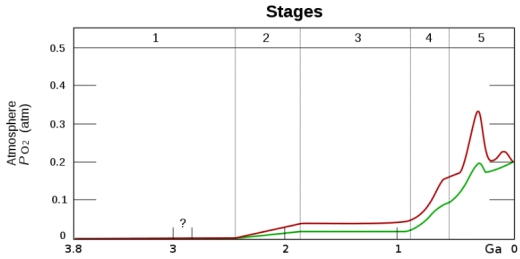
Image: Heinrich D. Holland derivative work: Loudubewe (talk) – Oxygenation-atm.svg, CC BY-SA 3.0,
https://commons.wikimedia.org/w/index.php?curid=12776502
With the absence of high partial pressures of O2 before the Pre-Cambrian, are there biogenic chemical disequilibrium conditions that can be discerned from the state of primordial atmospheres subject to purely abiotic equilibrium?
The new Krissansen-Totton et al? paper attempts to do that for the Archaean (4 – 2.5 gya) and Proterozoic (2.5 – 0.54) eons. Their approach is to calculate the Gibbs Free Energy (G), a metric of disequilibrium, for gases in an atmosphere-oceanic environment. The authors use a range of gas mixtures from the geologic record and determine the disequilibrium they represent using calculations of G for the observed versus the expected equilibrium concentrations of chemical species.
The authors note that almost all the G is in our ocean compartment from the nitrogen (N2)-O2 not reaching equilibrium as ionic nitrate. A small, but very important disequilibrium between methane (CH4) and O2 in the atmosphere is also considered a biosignature.
Using their approach, the authors look at the disequilibria in the atmosphere-ocean model in the earlier Archaean and Proterozoic eons. The geologic and model evidence suggests that the atmosphere was largely N2 and carbon dioxide (CO2), with a low concentration of O2 (2% or less partial pressure) in the Proterozoic.
In the Proterozoic, as today, the major disequilibrium is due to the lack of nitrate in the oceans and therefore the higher concentrations of O2 in the atmosphere. Similarly, an excess concentration of CH4 that should quickly oxidize to CO2 at equilibrium. In the Archaean, prior to the increase in O2 from photosynthesis, the N2, CO2, CH4 and liquid H2O equilibrium should consume the CH4 and increase the concentration of ammonium ions (NH4+ ) and bicarbonate (HCO3-) in the ocean. The persistence of CH4 in both eons is primarily driven by methanogen bacteria.
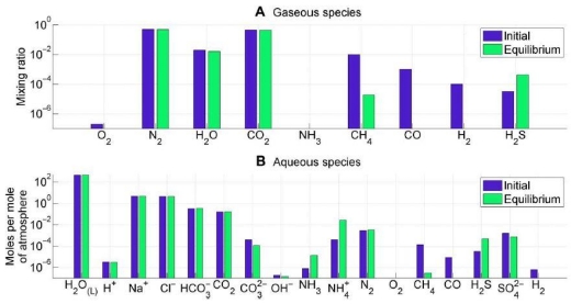
Image: Atmosphere-ocean disequilibrium in in the Archean. Blue bars denote assumed initial abundances from the literature, and green bars denote equilibrium abundances calculated using Gibbs free energy minimization. Subplots separate (A) atmospheric species and (B) ocean species. The most important contribution to Archean disequilibrium is the coexistence of atmospheric CH4, N2, CO2, and liquid water. These four species are lessened in abundance by reaction to equilibrium to form aqueous HCO3 and NH4. Oxidation of CO and H2 also contributes to the overall Gibbs energy change. Credit: Krissansen-Totton et al.
Therefore a biosignature for such an anoxic world in a stage similar to our Archaean era, would be to observe an ocean coupled with N2, CO2 and CH4 in the atmosphere. There is however an argument that might make this biosignature ambiguous.
CH4 and carbon monoxide (CO) might be present due to impacts of bolides (Kasting). Similarly, under certain conditions, it is possible that the mantle might be able to outgas CH4. In both cases, CO would be present and indicative of an abiogenic process. On Earth, CO is consumed as a substrate by bacteria, so its presence should be absent on a living world, even should such outgassing or impacts occur. The issue of CH4 outgassing, at least on earth, is countered by the known rates of outgassing compared to the concentration of CH4 in the atmosphere and ocean. The argument is primarily about rates of CH4 production between abiotic and biotic processes. Supporting Kasting, the authors conclude that on Earth, abiotic rates of production of CH4 fall far short of the observed levels.
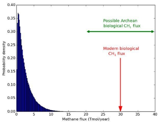
Image: Probability distribution for maximum abiotic methane production from serpentinization on Earth-like planets. This distribution was generated by sampling generous ranges for crustal production rates, FeO wt %, maximum fractional conversion of FeO to H2, and maximum fractional conversion of H2 to CH4, and then calculating the resultant methane flux 1 million times (see the main text). The modern biological flux (58) and plausible biological Archean flux (59) far exceed the maximum possible abiotic flux. These results support the hypothesis that the co-detection of abundant CH4 and CO2 on a habitable exoplanet is a plausible biosignature. Credit: Krissansen-Totton et al.
The authors conclude that their biosignature should also exclude the presence of CO to confirm the observed gases as a biosignature:
“The CH4-N2-CO2-H2O disequilibrium is thus a potentially detectable biosignature for Earth-like exoplanets with anoxic atmospheres and microbial biospheres. The simultaneous detection of abundant CH4 and CO2 (and the absence of CO) on an ostensibly habitable exoplanet would be strongly suggestive of biology.”
Given these gases in the presence of an ocean, can we use them to detect life on exoplanets?
Astronomers have been able to detect CO2, H2O, CH4 and CO in the atmosphere of HD 189733b, which is not Earthlike, but rather a hot Jupiter with a temperature of 1700F, far too hot for life. So far these gases have not been detectable on rocky worlds. Some new ground-based telescopes and the upcoming James Webb Space Telescope should have the capability of detecting these gases using transmission spectroscopy as these exoplanets transit their star.
It is important to note that the presence of an ocean is necessary to create high values of G. The Earth’s atmosphere alone has quite a low G, even compared to Mars. It is the presence of an ocean that results in G orders of magnitude larger than that from the atmosphere alone. Such an ocean is likely to be first detected by glints or the change in color of the planet as it rotates exposing different fractions of land and ocean.
An interesting observation of this approach is that a waterworld or ocean exoplanet might not show these biosignatures as the lack of weathering blocks the geologic carbon cycle and may preclude life’s emergence or long term survival. This theory might now be testable using spectroscopy and calculations for G.
This approach to biosignatures is applicable to our own solar system. As mentioned, Mars’ current G is greater than Earth’s atmosphere G. This is due to the photochemical disequilibrium of CO and O2. The detection of CH4 in Mars’ atmosphere, although at very low levels, would add to their calculation of Mars’ atmospheric G. In future, if the size of Mars’ early ocean can be inferred and gases in rocks extracted, the evidence for paleo life might be inferred. Fossil evidence of life would then confirm the approach.
Similarly, the composition of the plumes from Europa and Enceladus should also allow calculation of G for these icy moons and help to infer whether their subsurface oceans are abiotic or support life.
Within a decade, we may have convincing evidence of extraterrestrial life. If any of those worlds are not too distant, the possibility of studying that life directly in the future will be exciting.
The paper is Krissansen-Totton? et al., “Disequilibrium biosignatures over Earth history and implications for detecting exoplanet life,?” (2018)? Science Advances 4 ? (abstract? / ?full tex?t).
Streamlining Exoplanet Validation
Between Kepler and the ensuing K2 mission, we’ve had quite a haul of exoplanets. Kepler data have been used to confirm 2341 exoplanets, with NASA declaring 30 of these as being less than twice Earth-size and in the habitable zone. K2 has landed 307 confirmed worlds of its own. K2 offers a different viewing strategy than Kepler’s fixed view of over 150,000 stars. While the transit method is still at work, K2 pursues a series of observing campaigns, its fields of view distributed around the ecliptic plane, and with photometric precision approaching the original.
Why the relationship with the ecliptic? Remember that what turned Kepler into K2 was the failure of two reaction wheels, the second failing less than a year after the first. Working in the ecliptic plane minimizes the torque produced by solar wind pressure, thus minimizing pointing drift and allowing the spacecraft to be controlled by its thrusters and remaining two reaction wheels. Each K2 campaign is limited to about 80 days because of sun angle constraints.
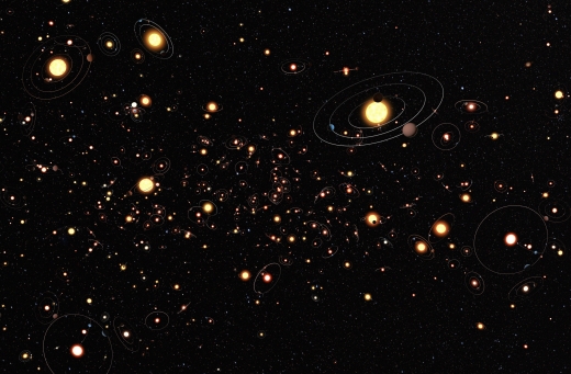
Image: After detecting the first exoplanets in the 1990s, astronomers have learned that planets around other stars are the rule rather than the exception. There are likely hundreds of billions of exoplanets in the Milky Way alone. Credit: ESA/Hubble/ESO/M. Kornmesser.
More K2 planets have now turned up in an international study led by Andrew Mayo (National Space Institute, Technical University of Denmark). The research, underway since the first release of K2 data in 2014, uncovered 275 planet candidates, of which 149 were validated. 56 of the latter had not previously been detected, while 39 had already been identified as candidates, and 53 had already been validated, with one previously classed as a false positive.
Overall, the work increases the validated K2 planet sample by almost 50 percent, while increasing the K2 candidate sample by 20 percent. What stands out here is not so much the trove of new planets but the validation techniques brought to bear, which were applied to a large sample as part of a framework developed to increase validation speed. From the paper:
This research will also be useful even after the end of the K2 mission. The upcoming TESS mission (Ricker et al. 2015) is expected to yield more than 1500 total exoplanet discoveries, but it is also estimated that TESS will detect over 1000 false positive signals (Sullivan et al. 2015). Even so, one (out of three) of the level one baseline science requirements for TESS is to measure the masses of 50 planets with Rp < 4 R?. Therefore, there will need to be an extensive follow-up program to the primary photometric observations conducted by the spacecraft, including careful statistical validation to aid in the selection of follow-up targets. The work presented here will be extremely useful in that follow-up program, since only modest adjustments will allow for the validation of planet candidate systems identified by TESS rather than K2.
The work involves not only analysis of the K2 light curves but also follow-up spectroscopy and high contrast imaging involving ground-based observation of candidate host stars. The processes of data reduction, candidate identification, and statistical validation described here using a statistical validation tool called vespa clearly have application well beyond K2.
The paper is Mayo et al., “275 Candidates and 149 Validated Planets Orbiting Bright Stars in K2 Campaigns 0-10,” accepted at the Astronomical Journal (preprint).
Computation Between the Stars

Frank Wilczek has used the neologism ‘quintelligence’ to refer to the kind of sentience that might grow out of artificial intelligence and neural networks using genetic algorithms. I seem to remember running across Wilczek’s term in one of Paul Davies books, though I can’t remember which. In any case, Davies has speculated himself about what such intelligences might look like, located in interstellar space and exploiting ultracool temperatures.
A SETI target? If so, how would we spot such a civilization?
Wilczek is someone I listen to carefully. Now at MIT, he’s a mathematician and theoretical physicist who was awarded the Nobel Prize in Physics in 2004, along with David Gross and David Politzer, for work on the strong interaction. He’s also the author of several books explicating modern physics to lay readers. I’ve read his The Lightness of Being: Mass, Ether, and the Unification of Forces (Basic Books, 2008) and found it densely packed but rewarding. I haven’t yet tackled 2015’s A Beautiful Question: Finding Nature’s Deep Design.
Perhaps you saw Wilczek’s recent piece in The Wall Street Journal, sent my way by Michael Michaud. Here we find the scientist going at the Fermi question that we have tackled so many times in these pages, always coming back to the issue that we have a sample of one when it comes to life in the universe, much less technological society, and our sample is right here on Earth. For the record, Wilczek doesn’t buy the idea that life is unusual; in fact, he states not only that he thinks life is common, but also makes the case for advanced civilizations:
Generalized intelligence, that produces technology, took a lot longer to develop, however, and the road from amoebas to hominids is littered with evolutionary accidents. So maybe we’re our galaxy’s only example. Maybe. But since evolution has supported many wild and sophisticated experiments, and because the experiment of intelligence brings spectacular adaptive success, I suspect the opposite. Plenty of older technological civilizations are out there.
Civilizations may, of course, develop and then, in Wilczek’s phrase, ‘flame out,’ just as Edward Gibbon would describe the fall of Rome as “the natural and inevitable effect of immoderate greatness. . . . The stupendous fabric yielded to the pressure of its own weight.” We can pile evidence onto that one, from the British and Spanish empires to the decline of numerous societies like the Aztec and the Mayan. Catastrophe is always a possible human outcome.
But is it an outcome for non-human technological societies? Wilczek doubts that, preferring to hark back to the idea with which we opened. The most advanced quantum computation — quintelligence — he believes, works best where it is cold and dark. And a civilization based on what we would today call artificial intelligence may be one that basically wants to be left alone.
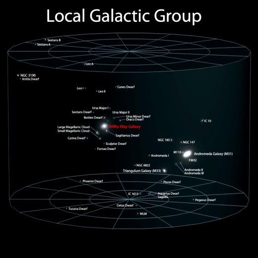
Image: The Local Group of galaxies. Is the most likely place for advanced civilization to be found in the immensities between stars and galaxies? Credit: Andrew Z. Colvin.
All this is, like all Fermi question talk, no more than speculation, but it’s interesting speculation, for Wilczek goes on to discuss the notion that one outcome for a hyper-advanced civilization may be to embrace the small. After all, the speed of light is a limit to communications, and effective computation involves communications that are affected by that limit. The implication: Fast AI thinking works best when it occurs in relatively small spaces. Thus:
Consider a computer operating at a speed of 10 gigahertz, which is not far from what you can buy today. In the time between its computational steps, light can travel just over an inch. Accordingly, powerful thinking entities that obey the laws of physics, and which need to exchange up-to-date information, can’t be spaced much farther apart than that. Thinkers at the vanguard of a hyper-advanced technology, striving to be both quick-witted and coherent, would keep that technology small.
A civilization based, then, on information processing would achieve its highest gains by going small in search of the highest levels of speed and integration. We’re now back out in the interstellar wastelands, which may in this scenario actually contain advanced and utterly inconspicuous intelligences. As I mentioned earlier, it’s hard to see how SETI finds these.
Unstated in Wilczek’s article is a different issue. Let’s concede the possibility of all but invisible hyper-intelligence elsewhere in the cosmos. We don’t know how long it would take to develop such a civilization, moving presumably out of its initial biological state into the realm of computation and AI. Surely along the way, there would still be societies in biological form leaving detectable traces of themselves. Or should we assume that the Singularity really is near enough that even a culture like ours may be succeeded by AI in the cosmic blink of an eye?
Probing Outer Planet Storms
A Hubble project called Outer Planet Atmospheres Legacy (OPAL) has been producing long-term information about the four outer planets at ultraviolet wavelengths, a unique capability that has paid off in deepening our knowledge of Neptune. If you kept pace with Voyager 2 at Neptune, you’ll recall that the spacecraft found huge dark storms in the planet’s atmosphere. Neptune proved to be more atmospherically active than its distance from the Sun would have suggested, and Hubble found another two storms in the mid-1990’s that later vanished.
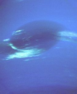
Image: Neptune’s Great Dark Spot, a large anticyclonic storm similar to Jupiter’s Great Red Spot, observed by NASA’s Voyager 2 spacecraft in 1989. The image was shuttered 45 hours before closest approach at a distance of 2.8 million kilometers. The smallest structures that can be seen are of an order of 50 kilometers. The image shows feathery white clouds that overlie the boundary of the dark and light blue regions. Credit: NASA/JPL.
Now we have evidence of another storm, discovered by Hubble in 2015 and evidently vanishing before our eyes. This is a storm that was once large enough to have spanned the Atlantic, evidently visible because primarily composed of hydrogen sulfide drawn up from the deeper atmosphere. UC-Berkeley’s Joshua Tollefson, a co-author on the new paper on this work, notes that the storm’s darkness is relative: “The particles themselves are still highly reflective; they are just slightly darker than the particles in the surrounding atmosphere.”
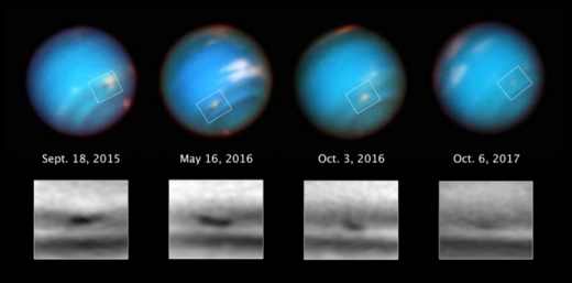
Image: This series of Hubble Space Telescope images taken over 2 years tracks the demise of a giant dark vortex on the planet Neptune. The oval-shaped spot has shrunk from 5,000 kilometers across its long axis to 3,700 kilometers across, over the Hubble observation period. Immense dark storms on Neptune were first discovered in the late 1980s by the Voyager 2 spacecraft. Since then only Hubble has tracked these elusive features. Hubble found two dark storms that appeared in the mid-1990s and then vanished. This latest storm was first seen in 2015. The first images of the dark vortex are from the Outer Planet Atmospheres Legacy (OPAL) program, a long-term Hubble project that annually captures global maps of our solar system’s four outer planets. Credit: NASA, ESA, and M.H. Wong and A.I. Hsu (UC Berkeley).
The differences between Neptune’s storms and famous Jovian features like the Great Red Spot are interesting though not yet fully understood. The Great Red Spot has been a well described feature on Jupiter for more than two centuries, still robust though varying in size and color. A storm that once encompassed four Earth diameters had shrunk to twice Earth’s diameter in the Voyager 2 flyby of 1979, and has now dropped to perhaps 1.3. As to its heat sources, they are still under investigation, as we saw in 2016 (check Jupiter’s Great Red Spot as Heat Source).
Neptune is another story, with storms that seem to last but a few years. Thus the fading of the recent dark spot, which had been observed at mid-southern latitudes. Michael H. Wong (UC-Berkeley) is lead author of the paper:
“It looks like we’re capturing the demise of this dark vortex, and it’s different from what well-known studies led us to expect. Their dynamical simulations said that anticyclones under Neptune’s wind shear would probably drift toward the equator. We thought that once the vortex got too close to the equator, it would break up and perhaps create a spectacular outburst of cloud activity.”
But the storm drifted not toward the equator but the south pole, not constrained by the powerful alternating wind jets found on Jupiter. Moreover, we have no information on how these storms form or how fast they rotate. And as the new paper notes, the five Neptune dark spots we’ve thus far found have differed broadly in terms of size, shape, oscillatory behavior and companion cloud distribution. We have much to learn about their formation, behavior and dissipation.
When you think about flyby missions like Voyager 2 at Neptune, the value of getting that first look at a hitherto unknown object is obvious. But we are moving into an era when longer-term observations become paramount. The OPAL program with Hubble is an example of this, studying in the case of Neptune a phenomenon that seems to exist on a timescale that suits an annual series of observations. Hubble has been complemented by observations from other observatories, including not just Spitzer but, interestingly, Kepler K2. A robotic adaptive optics system tuned for planetary atmospheric science is being prepared for deployment in Hawaii, offering a way to scrutinize these worlds over even smaller periods.
From the paper:
Clearly, there is much room in the discovery space of solar system time domain science. There is room in this discovery space for exploration by a dedicated solar system space telescope, a network of ground facilities, and cadence programs at astrophysical observatories with advanced capabilities.
The paper is Wong et al., “A New Dark Vortex on Neptune,” Astronomical Journal Vol. 155, No. 3 (15 February 2018). Abstract.
Mistakes in the Drake Equation
Juggling all the factors impacting the emergence of extraterrestrial civilizations is no easy task, which is why the Drake equation has become such a handy tool. But are there assumptions locked inside it that need examination? Robert Zubrin thinks so, and in the essay that follows, he explains why, with a particular nod to the possibility that life can move among the stars. Although he is well known for his work at The Mars Society and authorship of The Case for Mars, Zubrin became a factor in my work when I discovered his book Entering Space: Creating a Spacefaring Civilization back in 2000, which led me to his scientific papers, including key work on the Bussard ramjet concept and magsail braking. Today’s look at Frank Drake’s equation reaches wide-ranging conclusions, particularly when we begin to tweak the parameters affecting both the lifetime of civilizations and the length of time it takes them to emerge and spread into the cosmos.
by Robert Zubrin

There are 400 billion other solar systems in our galaxy, and it’s been around for 10 billion years. Clearly it stands to reason that there must be extraterrestrial civilizations. We know this, because the laws of nature that led to the development of life and intelligence on Earth must be the same as those prevailing elsewhere in the universe.
Hence, they are out there. The question is: how many?
In 1961, radio astronomer Frank Drake developed a pedagogy for analyzing the question of the frequency of extraterrestrial civilizations. According to Drake, in steady state the rate at which new civilizations form should equal the rate at which they pass away, and therefore we can write:
![]()
Equation (1) is therefore known as the “Drake Equation.” Herein, N is the number of technological civilizations is our galaxy, and L is the average lifetime of a technological civilization. The left-hand side term, N/L, is the rate at which such civilizations are disappearing from the galaxy. On the right-hand side, we have R?, the rate of star formation in our galaxy; fp, the fraction of these stars that have planetary systems; ne, is the mean number of planets in each system that have environments favorable to life; fl the fraction of these that actually developed life; fi the fraction of these that evolved intelligent species; and fc the fraction of intelligent species that developed sufficient technology for interstellar communication. (In other words, the Drake equation defines a “civilization” as a species possessing radiotelescopes. By this definition, civilization did not appear on Earth until the 1930s.)
By plugging in numbers, we can use the Drake equation to compute N. For example, if we estimate L=50,000 years (ten times recorded history), R? = 10 stars per year, fp = 0.5, and each of the other four factors ne, fl, fi, and fc equal to 0.2, we calculate the total number of technological civilizations in our galaxy, N, equals 400.
Four-hundred civilizations in our galaxy may seem like a lot, but scattered among the Milky Way’s 400 billion stars, they would represent a very tiny fraction: just one in a billion to be precise. In our own region of the galaxy, (known) stars occur with a density of about one in every 320 cubic light years. If the calculation in the previous paragraph were correct, it would therefore indicate that the nearest extraterrestrial civilization is likely to be about 4,300 light years away.
But, classic as it may be, the Drake equation is patently incorrect. For example, the equation assumes that life, intelligence, and civilization can only evolve in a given solar system once. This is manifestly untrue. Stars evolve on time scales of billions of years, species over millions of years, and civilizations take mere thousands of years.
Current human civilization could knock itself out with a thermonuclear war, but unless humanity drove itself into complete extinction, there is little doubt that 1,000 years later global civilization would be fully reestablished. An asteroidal impact on the scale of the K-T event that eliminated the dinosaurs might well wipe out humanity completely. But 5 million years after the K-T impact the biosphere had fully recovered and was sporting the early Cenozoic’s promising array of novel mammals, birds, and reptiles. Similarly, 5 million years after a K-T class event drove humanity and most of the other land species to extinction, the world would be repopulated with new species, including probably many types of advanced mammals descended from current nocturnal or aquatic varieties.
Human ancestors 30 million years ago were no more intelligent than otters. It is unlikely that the biosphere would require significantly longer than that to recreate our capabilities in a new species. This is much faster than the 4 billion years required by nature to produce a brand-new biosphere in a new solar system. Furthermore, the Drake equation also ignores the possibility that both life and civilization can propagate across interstellar space.
So, let’s reconsider the question.
Estimating the Galactic Population
There are 400 billion stars in our galaxy, and about 10 percent of them are good G and K type stars which are not part of multiple stellar systems. Almost all of these probably have planets, and it’s a fair guess that 10 percent of these planetary systems feature a world with an active biosphere, probably half of which have been living and evolving for as long as the Earth. That leaves us with two billion active, well-developed biospheres filled with complex plants and animals, capable of generating technological species on time scales of somewhere between 10 and 40 million years. As a middle value, let’s choose 20 million years as the “regeneration time” tr. Then we have:
![]()
where N and L are defined as in the Drake equation, and ns is the number of stars in the galaxy (400 billion), fg is the fraction of them that are “good” (single G and K) type stars (about 0.1), fb is the fraction of those with planets with active biospheres (we estimate 0.1), fm is the fraction of those biospheres that are “mature” (estimate 0.5), and nb, the product of these last four factors, is the number of active mature biospheres in the galaxy.
If we stick with our previous estimate that the lifetime, L, of an average technological civilization is 50,000 years, and plug in the rest of the above numbers, equation (2) says that there are probably 5 million technological civilizations active in the galaxy right now. That’s a lot more than suggested by the Drake equation. Indeed, it indicates that one out of every 80,000 stars warms the home world of a technological society. Given the local density of stars in our own region of the galaxy, this implies that the nearest center of extraterrestrial civilization could be expected at a distance of about 185 light years.
Technological civilizations, if they last any time at all, will become starfaring. In our own case (and our own case is the only basis we have for most of these estimations), the gap between development of radiotelescopes and the achievement of interstellar flight is unlikely to span more than a couple of centuries, which is insignificant when measured against L=50,000 years. This suggests that once a civilization gets started, it’s likely to spread. Propulsion systems capable of generating spacecraft velocities on the order of 5 percent the speed of light appear possible. However, interstellar colonists will probably target nearby stars, with further colonization efforts originating in the frontier stellar systems once civilization becomes sufficiently well-established there to launch such expeditions.
In our own region of the galaxy, the typical distance between stars is five or six light years. So, if we guess that it might take 1,000 years to consolidate and develop a new solar system to the point where it is ready to launch missions of its own, this would suggest the speed at which a settlement wave spreads through the galaxy might be on the order of 0.5 percent the speed of light. However, the period of expansion of a civilization is not necessarily the same as the lifetime of the civilization; it can’t be more, and it could be considerably less. If we assume that the expansion period might be half the lifetime, then the average rate of expansion, V, would be half the speed of the settlement wave, or 0.25 percent the speed of light.
As a civilization expands, its zone of settlement encompasses more and more stars. The density, d, of stars in our region of the galaxy is about 0.003 stars per cubic light year, of which a fraction, fg, of about 10 percent are likely to be viable potential homes for life and technological civilizations. Combining these considerations with equation 2, we can create a new equation to estimate C, the number of civilized solar systems in our galaxy, by multiplying the number of civilizations N, by, nu, the average number of useful stars available to each.
![]()
For example, we have assumed that the average lifespan, L, of a technological species is 50,000 years, and if that is true, then the average age of one is half of this, or 25,000 years. If a typical civilization has been spreading out at the above estimated rate for this amount of time, the radius, R, of its settlement zone would be 62.5 light years (R = VL/2 = 62.5 ly), and its domain would include about 3,000 stars. If we multiply this domain size by the number of expected civilizations calculated above, we find that about 15 billion stars, or 3.75 percent of the galactic population, would be expected to lie within somebody’s sphere of influence. If 10 percent of these stars are actually settled, this implies there are about 1.5 billion civilized stellar systems within our galaxy. Furthermore, we find that the nearest outpost of extraterrestrial civilization could be expected to be found at a distance of 185-62.5 = 122.5 light years.
The above calculation represents my best guess as to the shape of things, but there’s obviously a lot of uncertainty in the calculation. The biggest uncertainty revolves around the value of L; we have very little data to estimate this number and the value we pick for it strongly influences the results of the calculation. The value of V is also rather uncertain, although less so than L, as engineering knowledge can provide some guide. In Table 1 we show how the answers might change if we take alternative values for L and V, while keeping the other assumptions we have adopted constant.
Table 1 The Number and Distribution of Galactic Civilizations
| V=0.005 c | V=0.0025 c | V=0.001 c | |
| L=10,000 years | |||
| N (# civilizations) | 1 million | 1 million | 1 million |
| C (# civilized stars) | 19.5 million | 2.4 million | 1 million |
| R (radius of domain) | 25 ly | 12.5 ly | 5 ly |
| S (Separation between civilizations) | 316 ly | 316 ly | 316 ly |
| D (distance to nearest outpost) | 291 ly | 304 ly | 311 ly |
| F (fraction of stars within domains) | 0.048% | 0.006% | 0.0025% |
| L=50,000 years | |||
| N (# civilizations) | 5 million | 5 million | 5 million |
| C (# civilized stars) | 12 billion | 1.5 billion | 98 million |
| R (radius of domain) | 125 ly | 62.5 ly | 25 ly |
| S (Separation between civilizations) | 185 ly | 185 ly | 185 ly |
| D (distance to nearest outpost) | 60 ly | 122.5 ly | 160 ly |
| F (fraction of stars within domains) | 30% | 3.75% | 0.245% |
| L=200,000 years | |||
| N (# civilizations) | 20 million | 20 million | 20 million |
| C (# civilized stars) | 40 billion | 40 billion | 18 billion |
| R (radius of domain) | 500 ly | 250 ly | 100 ly |
| S (Separation between civilizations) | 131 ly | 131 ly | 131 ly |
| D (distance to nearest outpost) | 0 ly | 0 ly | 31 ly |
| F (fraction of stars within domains) | 100% | 100% | 44% |
In Table 1, N is the number of technological civilizations in the galaxy (5 million in the previous calculation) , C is the number of stellar systems that some civilization has settled (1.5 billion, above), R is the radius of a typical domain (62.5 ly above), S is the separation distance between the centers of civilization (185 ly above), D is the probable distance to the nearest extraterrestrial outpost (122.5 ly, above), and F is the fraction of the stars in the galaxy that are within someone’s sphere of influence (3.75% above).
Examining the numbers in Table 1, we can see how the value of L completely dominates our picture of the galaxy. If L is “short” (10,000 years or less), then interstellar civilizations are few and far between, and direct contact would almost never occur. If L is “medium” (~50,000 years), then the radius of domains is likely to be smaller than the distance between civilizations, but not much smaller, and so contact could be expected to happen occasionally (remember, L, V, and S are averages; particular civilizations in various localities could vary in their values for these quantities). If L is a long time (> 200,000 years), then civilizations are closely packed, and contact should occur frequently. (These relationships between L and the density of civilizations apply in our region of the galaxy. In the core, stars are packed tighter, so smaller values of L are needed to produce the same “packing fraction,” but the same general trends apply.)
Any way you slice it, one thing seems rather certain: There’s plenty of them out there.
What are these civilizations like? What have they achieved?
It would be good to know.

Follow with RSS or E-Mail
