Centauri Dreams
Imagining and Planning Interstellar Exploration
Recovering a Triple Star Planet with New Data
The Kepler mission produced so much data — 2394 exoplanets, 2366 candidates by the end of spacecraft operations in 2018 — that we might forget how quickly all this came about. The first Kepler results started being announced in 2010. One of these, the second candidate to emerge, was KOI-5Ab, which was a tough pick in the early going given its position within a triple star system. An ambiguous detection, it was soon left behind, its status uncertain, as the numbers of more definitive candidates swelled. Caltech’s David Ciardi, who discussed this elusive system at the recent virtual meeting of the American Astronomical Society, says this about it:
“KOI-5Ab got abandoned because it was complicated, and we had thousands of candidates. There were easier pickings than KOI-5Ab, and we were learning something new from Kepler every day, so that KOI-5 was mostly forgotten.”
Ciardi, who is chief scientist at NASA’s Exoplanet Science Institute, has now pulled KOI-5Ab back to vibrant life. Almost certainly a gas giant, the planet orbits one of three stars in the system in a misaligned orbit that calls into question the nature of its formation. Making original confirmation of the planet difficult was the inability to completely distinguish it from the possible effects of the other two stars in the system. Untangling the question would involve TESS data. The object appears in TESS terminology as TOI-1241b, showing a five-day orbit that matches the Kepler result.
Confirming such a candidate calls for more than a single backup asset on the ground. Working with colleagues in the California Planet Search, Ciardi used Keck data, as well as observations from Caltech’s Palomar Observatory near San Diego and Gemini North in Hawaii, though the scientist credits TESS as the motivation for re-visiting the object. We learn that KOI-5Ab orbits Star A, whose companion, Star B, is in a tight 30 year orbit with A. The third star orbits A and B every 400 years. Have a look at the image below to see the orbital dance.
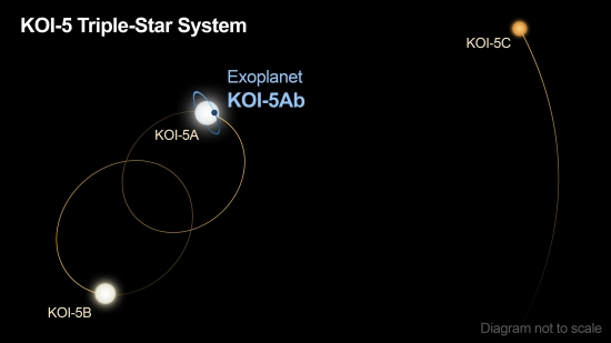
Image: The KOI-5 star system consists of three stars, labeled A, B, and C in this diagram. Star A and B orbit each other every 30 years. Star C orbits stars A and B every 400 years. The system hosts one known planet, called KOI-5Ab, which was discovered and characterized using data from NASA’s Kepler and TESS (Transiting Exoplanet Survey Satellite) missions, as well as ground-based telescopes. KOI-5Ab is about half the mass of Saturn and orbits star A roughly every five days. Its orbit is titled 50 degrees relative to the plane of stars A and B. Astronomers suspect that this misaligned orbit was caused by star B, which gravitationally kicked the planet during its development, skewing its orbit and causing it to migrate inward. Credit: Caltech/R. Hurt (IPAC).
The orbital mechanics in play as planets formed from a primordial disk could account for the misalignment, given the gravitational influence of the second star, causing the planet to migrate inward as well as skewing its inclination. There are similar cases of misaligned orbits — particular GW Orionis — offering evidence of distortions caused by multiple star system evolution.
“We don’t know of many planets that exist in triple-star systems, and this one is extra special because its orbit is skewed,” adds Ciardi. “We still have a lot of questions about how and when planets can form in multiple-star systems and how their properties compare to planets in single-star systems. By studying this system in greater detail, perhaps we can gain insight into how the universe makes planets.”
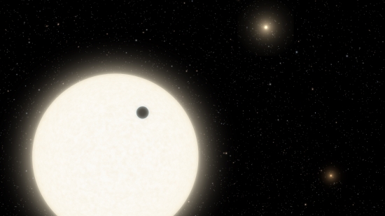
Image: This artist’s concept shows the planet KOI-5Ab transiting across the face of a sun-like star, which is part of a triple-star system located 1,800 light-years away in the constellation Cygnus. Credit: Caltech/R. Hurt (IPAC).

Across the Brown Dwarf Palette
Something to note about the brown dwarfs we looked at yesterday: Our views on how they would appear to someone nearby in visible light are changing. It’s an interesting issue because these brown dwarfs exist in more than a single type. If you’ll have a look at the image below, you’ll see a NASA artist conception of the three classes of brown dwarf, all of these being objects that lack the mass to burn with sustained fusion.
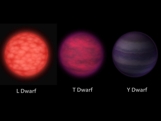
Image: This artist’s conception illustrates what brown dwarfs of different types might look like to a hypothetical interstellar traveler who has flown a spaceship to each one. Brown dwarfs are like stars, but they aren’t massive enough to fuse atoms steadily and shine with starlight — as our sun does so well. Our thoughts on how these objects appear are evolving quickly, as witness yesterday’s discussion, and we’re likely to need another visual rendering of brown dwarf classes soon. Credit: NASA/JPL-Caltech.
One thing should jump out to anyone who read yesterday’s post on the appearance of Luhman 16 B: The artist here does not depict bands of clouds/weather on the object, but rather localized storms of the kind that some researchers believed would characterize brown dwarfs. We know that Luhman 16 A (33 times Jupiter’s mass) is of spectral type L7.5, while Luhman 16 B is categorized as T0.5, putting it near the transition between types L and T. And Luhman 16 B shows strong evidence of banding.
That’s according to Daniel Apai and team, as discussed yesterday, in an analysis based on data from TESS. Looking further at the image above, it’s clear we’re going to be re-working our depictions going forward as we analyze more brown dwarfs. If we should expect a banded object at the L-T transition, then at least the L dwarf and the T dwarf shown here will likely show the same atmospheric pattern (obviously, we’ll need to confirm these speculations with hard data). That would leave the Y dwarf as yet undetermined, and for good reason, as these objects are vanishingly hard to see.
Atmospheric temperatures drop as we move across the types of brown dwarfs here, with the L dwarf being the brightest and hottest in the image; its typical temperatures are in the range of 1400 degrees Celsius. The magenta T dwarf takes us down to about 900 degrees Celsius, but the Y dwarf really drops the reading, with the coldest yet identified having a temperature of a mere 25 degrees Celsius. That’s not all that far off what my thermostat is set on — 72 ? — as I try to take the chill off this morning.
All three of the brown dwarfs shown above appear at the same size, a reminder that all types of this object have the same dimension, which is roughly that of Jupiter, despite wide variations in their mass. Same radius, major disparity in mass, in other words. My hopes that we would find one of these fascinating objects at no more than, say, 1 light year seem to have been dashed, although it’s certainly true that Y dwarfs are so cool that finding them is going to be difficult even for the best infrared observatories.
As we keep looking, we can now refer to the updated map of L, T and Y dwarfs in the vicinity of the Solar System that the Backyard Worlds: Planet 9 project has produced. You’ll recall from earlier posts here that Backyard Worlds: Planet 9 is funded by NASA as a collaboration between professional scientists and the public.
All those non-professional but often highly adept astronomers and volunteers have produced a map with a radius of about 65 light years. The work of 150,000 volunteers has been going on since 2017 using data from the WISE mission under its Near-Earth Object Wide-Field Infrared Survey Explorer (NEOWISE) incarnation. The study was presented at the ongoing virtual meeting of the American Astronomical Society.
Dozens of new brown dwarfs turned up in this work, which drew on data from the now retired Spitzer Space Telescope. Using the Backyard Worlds: Planet 9 results, astronomers consulted data from the space telescope to observe 361 local brown dwarfs of types L, T and Y and combined the results with previously known dwarfs, many of them catalogued by CatWise, the catalog of objects from WISE and NEOWISE.
The result: a 3D map of 525 brown dwarfs.
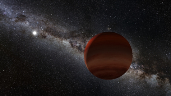
Image: In this artist’s rendering, the small white orb represents a white dwarf (a remnant of a long-dead Sun-like star), while the purple foreground object is a newly discovered brown dwarf companion, confirmed by NASA’s Spitzer Space Telescope. This faint brown dwarf was previously overlooked until being spotted by citizen scientists working with Backyard Worlds: Planet 9, a NASA-funded citizen science project. Credits: NOIRLab/NSF/AURA/P. Marenfeld/Acknowledgement: William Pendrill.
The galaxy’s coldest known Y dwarf is a neighbor (not surprising, given that more distant dwarfs should be below the level of detection), but it turns out that it is comparatively rare, a bit of an anomaly given our expectations of brown dwarf distribution. Of the seven objects nearest to our Solar System, three are brown dwarfs. And the Sun’s position within this cluster of nearby objects is a bit unusual as well, says Aaron Meisner (National Science Foundation NOIRLab), a co-author of the study:
“If you were to put the Sun at a random place within our 3D map and you were to ask, ‘Typically, what do its neighbors look like?’ We find that they would look very different from what our actual neighbors are.”
Again, we have to weigh this outcome against the difficulty in observing Y dwarfs, so conclusions shouldn’t be drawn too hastily. With brown dwarfs having exoplanet dimensions but no companion main sequence star (in most cases), they become useful objects as we refine the tools of exoplanet characterization. The James Webb Space Telescope should be able to tell us more about nearby brown dwarfs, as will the upcoming SPHEREx mission, an all-sky infrared survey scheduled for a 2024 launch.
The paper is Marocco et al., “The CatWISE2020 Catalog,” accepted for publication in the Astrophysical Journal Supplement Series (abstract/preprint).

What Does the Closest Brown Dwarf Look Like?
I keep hoping we’ll find a brown dwarf closer to us than Alpha Centauri, but none have turned up yet despite the best efforts of missions like WISE (Wide-Field Infrared Survey Explorer). If there’s something out there, it’s dim indeed. Of course, I wouldn’t be surprised at finding rogue planets between us and the nearest stars. Maybe some will be more massive than Jupiter, but evidently not massive enough to throw an infrared signature of the sort that defines a brown dwarf. Just what lies outside our system’s edge always makes for interesting speculation.
The beauty of finding an actual brown dwarf as opposed to a rogue planet is that we might be dealing with a planetary system in miniature, a fine target in our own backyards. Lacking that, the closest brown dwarf we know is the Luhman 16 AB system, a binary in the southern constellation of Vela some 6.5 light years from the Sun (a little further than Barnard’s Star, making this the third closest known system to the Sun). Here we have one dwarf about 34 times Jupiter’s mass (Luhman 16 A), and another, Luhman 16 B, about 28 times more massive than Jupiter, and because both are brown dwarfs, both are hotter than the planet.
Luhman 16 AB is the subject of a new paper from Daniel Apai (University of Arizona / Lunar and Planetary Laboratory). Apai’s team was intent on finding out what brown dwarfs look like, wondering whether they’d be marked by the kind of well-defined banding and belts we see on Jupiter or roiling with storms of the kind we’ve seen (thanks to Juno) on Jupiter’s poles. The method: Using data from TESS (Transiting Exoplanet Survey Satellite), the researchers deployed in-house algorithms to measure brightness changes of the two brown dwarfs as they rotated. Brighter atmospheric features rotate in and out of view.
What emerged was the most detailed look yet at a brown dwarf’s atmospheric circulation, and that led to conclusions about the appearance of these objects. We now know that Jupiter is a good analogy for what we would see if we could look at Luhman 16 AB up close. The work created a model for Luhman 16 B’s atmosphere showing that high-speed winds run parallel to the brown dwarf’s equator. Also like Jupiter are the apparent vortices emerging in the polar regions. Here we need to pause to thank the late Adam Showman, also of the University of Arizona, whose models predicted this pattern.
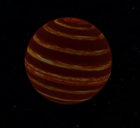
Image: Using high-precision brightness measurements from NASA’s TESS space telescope, astronomers found that the nearby brown dwarf Luhman 16 B’s atmosphere is dominated by high-speed, global winds akin to Earth’s jet stream system. This global circulation determines how clouds are distributed in the brown dwarf’s atmosphere, giving it a striped appearance. Credit: Daniel Apai.
The lighter zones shown above are thought to be thin cloud decks illuminated by light from the hot interior, while the darker zones are where thicker cloud decks block interior light. The wind speeds are highest at the equator, dropping at the higher latitudes. The global wind pattern is lost at the poles, which are a region of enormous local storms, as on Jupiter. Most of Luhman 16 B, then, is dominated by global wind patterns rather than localized storms.
Something of a surprise to the team (the paper refers to the development as ‘a stunning feature’) is the changeable, non-periodic nature of the Luhman 16 light curve. Here’s how the authors describe this fact:
…we identify four properties that are shared between the visual lightcurve of this object and the infrared lightcurves of other objects: 1) The lightcurves remain variable over long periods (years); 2) The lightcurve shape evolves, yet it displays characteristic period, which is likely the rotational period of the object (as found in Apai et al. 2017); 3) In spite of the rapid evolution of the lightcurve, the amplitudes over rotational time-scales remain similar and characteristic to the object; 4) The lightcurves tend to be symmetric in the sense of similar amount of positive-negative features, in contrast to, for example, a situation in which a single positive feature appears periodically on an otherwise flat lightcurve, which would indicate a single bright spot in the atmosphere.
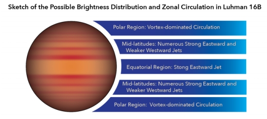
Image: This is Figure 16 from the paper. Caption: Sketch of the possible appearance of Luhman 16B, based on the emerging evidence. Zonal circulation models and comparison to Jupiter suggests that low-latitude regions are dominated by the fastest jets, and that wind speeds at mid-latitude are significantly lower. Circulation at the polar regions is likely to be vortex- and not jet-dominated. Cloud cover is likely to be correlated with the atmospheric circulation. Credit: Apai et al.
All this is drawn from TESS lightcurves of Luhman 16 AB covering 22 days and 100 rotations of the binary, allowing the researchers to conclude that both the brown dwarfs in this system show zonal circulation and fit the Jupiter model. It seems apparent that brown dwarfs can serve as more massive analogs of giant exoplanets and could thus help us develop techniques of atmospheric analysis that can be deployed even further from the Solar System. Says Apai:
“No telescope is large enough to provide detailed images of planets or brown dwarfs. But by measuring how the brightness of these rotating objects changes over time, it is possible to create crude maps of their atmospheres – a technique that, in the future, could also be used to map Earthlike planets in other solar systems that might otherwise be hard to see… Our study provides a template for future studies of similar objects on how to explore – and even map – the atmospheres of brown dwarfs and giant extrasolar planets without the need for telescopes powerful enough to resolve them visually.”
The paper is Apai et al. “TESS Observations of the Luhman 16 AB Brown Dwarf System: Rotational Periods, Lightcurve Evolution, and Zonal Circulation,” Astrophysical Journal Vol. 906, No. 1 (7 January 2021). Abstract / preprint.
Juno at Jupiter: Extended Mission Flybys of Galilean Moons
The news that NASA will extend the InSight mission on Mars for two years, taking it through December of 2022, is not surprising, given the data trove the mission team has collected through operation of the mission seismometer. A live asset on Mars also deepens our knowledge of the planet’s atmosphere and magnetic field, all reasons enough for pushing for another two years. But the extension of the Juno mission to Jupiter deserves more attention than it’s getting, given that Juno’s remit will be expanded deep into the Jovian system.

Image: NASA has extended both the Juno mission at Jupiter through September 2025 and the InSight mission at Mars through December 2022. Credit: NASA/JPL-Caltech.
For those of us fascinated with the outer system, this is good news indeed. I’m looking over two documents, the first being a presentation based on a report submitted to NASA’ Outer Planets Assessment Group (thanks to Ashley Baldwin for passing this along). The OPAG document was produced by Scott Bolton (Southwest Research Institute); it gives the overview of what a mission extension could look like. Also on my desk this morning is the text of the 2020 Planetary Missions Senior Review (PMSR), outlining a set of three mission scenarios. The context of both analyses is the success of the mission in studying Jupiter’s interior structure, magnetic field and magnetosphere, not to mention the examination of its atmospheric dynamics, seen in such roiling imagery as that depicted with stunning complexity in many of the JunoCam images.
Launched in 2011 and operational at Jupiter since 2016, Juno’s prime missions were to have ended in July of this year, with the spacecraft having completed 34 polar orbits, each of 53 day duration. The OPAG report refers to the subsequent extended mission as “a full Jovian system explorer with close flybys of satellites and rings.” The extended mission is to last through September, 2025, with observations of the planet’s ring system, its large moons, and a series of targeted observations and close flybys of Ganymede, Europa and Io.
That last clause really got my attention, as I hadn’t seen it coming. Juno is in an elliptical orbit with a 53-day period whose perijove migrates northward. This bit from the Senior Review reveals in depth the interactions between the various mission scenarios and satellite flybys. The three scenarios mentioned offer alternatives given varying science and budget considerations:
The proposed Juno extended mission (EM) would take advantage of the natural northward progression of the periapsis of the spacecraft’s orbit and the consequent lowering of spacecraft altitudes over Jupiter’s high northern latitudes. The EM would run until the end of the mission, with an expected duration of approximately four years. Under the High and Medium Scenarios, propulsive maneuvers would be utilized not only to target Jupiter-crossing longitude and perijove altitude, as during the prime mission, but also to target close flybys of Ganymede, Europa, and Io. The flyby maneuvers would act to shorten the spacecraft orbital period, yielding more close passes of Jupiter within a given time interval, and increase the rate of northward movement of spacecraft perijove. Under the Low scenario for EM operation, the satellite gravity assists and close satellite flybys would not be attempted.
So mission scientists have a number of options to work with. The extended mission investigates the northern hemisphere and probes the region above Jupiter’s polar cap aurora. The northern adjustment in Juno’s orbit is what makes the satellite flybys possible and enables as well close analysis of its ring structures. The Juno team can look forward to 3D mapping of Jupiter’s polar cyclones and studies of the planet’s unusual dilute core, the latter an earlier Juno discovery revealing a core consisting of both rocky material and ice as well as hydrogen and helium.
Both Europa Clipper and the European Space Agency’s JUICE mission (Jupiter Icy Moons Explorer) should benefit from Juno data on the radiation environment they will operate within. At Europa, Juno will continue the search for possible plume activity while examining the ice shell and mapping surface features, while studies of Io’s magma, polar volcanoes and interactions with Jupiter’s magnetosphere will be enabled by its encounters there. At Ganymede, magnetospheric interactions and surface composition data should be produced in abundance.
In the OPAG presentation, most of the Juno flybys will be at Io, with 11 possible between mid-2022 and 2025. Two encounters are planned for Ganymede (and recall that JUICE is scheduled to orbit the huge moon), and three encounters are feasible for Europa. The actual number of flybys will, according to the Senior Review, depend upon budget choices. In that document, I find this overview of Juno’s satellite flybys:
The orbit of Juno in the EM [extended mission] would take the spacecraft through the Io and Europa plasma tori and in close proximity to Io, Europa and Ganymede. Maps of Ganymede’s surface composition would allow studies to understand the importance of radiolytic processes in surface weathering, identify changes since Voyager and Galileo, and search for new craters. Juno’s Microwave Radiometer (MWR) is particularly sensitive to the upper 10 km of Europa’s ice shell. Studies at wavelengths complementing expected results from Europa Clipper’s radar would identify regions of thick and thin ice and search for regions where shallow subsurface liquid may exist. Juno’s visible and low-light cameras would search Europa for active plumes and changes in color/albedo that may reveal eruption regions since Galileo. The fields and particles experiments would look for evidence of recent activity. Finally, the Juno EM would include a flyby of Io and search for evidence of a magma ocean.
What an interesting development Juno’s extended mission turns out to be! Continuing science operations with existing equipment far undercuts the cost of new missions while extending long-duration datasets and, in the case of Juno, enabling a set of exciting new targets. We have the option here of a series of Galilean moon flybys that were never in Juno’s original mission, observations that could inform later choices made for Europa Clipper and JUICE. All told, Juno’s unanticipated extended mission is a heartening contribution to outer system science.
Hayabusa2: Multiple Paths for Analyzing an Asteroid
Ryugu is classified as a carbonaceous, or C-type asteroid, a class of objects thought to incorporate water-bearing minerals and organic compounds. Carbonaceous chondrites, the dark carbon-bearing meteorites found on Earth, are thought to originate in such asteroids, but it has been difficult if not impossible to determine the source of most individual meteorites.
Hence the significance of the Hayabusa2 mission. JAXA’s successful foray to Ryugu represents the first time we’ve been able to examine a sample of a C-type asteroid through direct collection at the site. Ralph Milliken is a planetary scientist at Brown University, where NASA maintains its Reflectance Experiment Laboratory (RELAB). The laboratory expects samples collected at Ryugu to arrive in short order. Milliken is interested in the history of water in the object:
“One of the things we’re trying to understand is the distribution of water in the early solar system, and how that water may have been delivered to Earth. Water-bearing asteroids are thought to have played a role in that, so by studying Ryugu up close and returning samples from it, we can better understand the abundance and history of water-bearing minerals on these kinds of asteroids.”
Milliken is also one of many co-authors on a new paper in Nature Astronomy looking at the thermal history of subsurface materials exposed on Ryugu. The paper examines data the spacecraft collected during its operations there, which can now be compared to the sample collection. We learn that the asteroid may not be as water-rich as originally thought, leading to various scenarios about how it might have lost its water. High on the list of possibilities is that this ‘rubble pile’ asteroid — essentially loose rock maintaining its shape because of gravity — dried after a collision or other disruption and subsequent reformation.
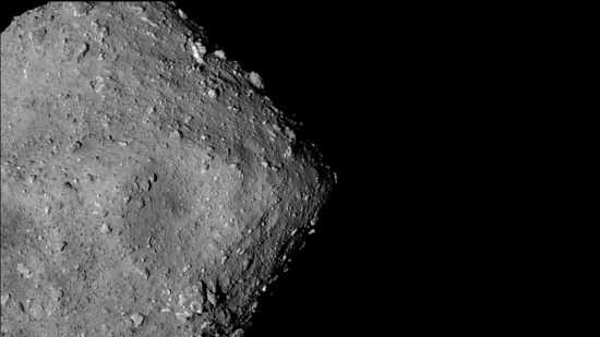
Image: Japan’s Hayabusa2 spacecraft snapped pictures of the asteroid Ryugu while flying alongside it two years ago. The spacecraft later returned rock samples from the asteroid to Earth. Credit: JAXA.
Bear in mind how Hayabusa2 proceeded with its sampling at Ryugu. During the 2019 rendezvous, the spacecraft fired a projectile into the asteroid’s surface that exposed the subsurface rock examined here. A near-infrared spectrometer was used to compare the water content of the surface with the material below, showing the two to be similar in water content. The authors see that as a clue that Ryugu’s parent body dried out, rather than the surface of Ryugu being dried out by the Sun, perhaps in a close solar pass earlier in its history.
In other words, heating by the Sun in one or more close solar passes would be likely to occur at the surface, without penetrating deep into the asteroid. What Hayabusa2’s spectrometer shows is that surface and sub-surface are both comparatively dry, which is an indication that it was the parent body of Ryugu, rather than an event happening to Ryugu itself, that produced this result.
Ahead for the Ryugu analysis is the need to study the size of the particles excavated from below the surface, which could play a role in how the spectrometer measurements are interpreted.
“The excavated material may have had a smaller grain size than what’s on the surface,” says Takahiro Hiroi, a senior research associate at Brown and another study co-author. “That grain size effect could make it appear darker and redder than its coarser counterpart on the surface. It’s hard to rule out that grain-size effect with remote sensing.”
The beauty of the successful sample return is that hypotheses about Ryugu’s past can now be evaluated through comparison of the remote sensing data and actual laboratory work. These are exciting times indeed for the scientists studying the extensive collection of asteroid debris Hayabusa 2 brought back. We can expect significant papers on all this in 2021.
The paper is Kitazato et al., “Thermally altered subsurface material of asteroid (162173) Ryugu,” Nature Astronomy 4 January 2021 (abstract).
The Red Dwarf Habitable Zone Dilemma
Henry Cordova, whose recent critique of traditional SETI kicked off a lengthy discussion in these pages, has been mulling over issues of habitability in the galaxy’s vast population of red dwarf stars. While we’ve focused on the questions raised by stellar flare activity and the climate challenges of tidal lock, the narrow band of habitability among the fainter M-dwarfs poses its own problems. How big a factor is a narrow circumstellar habitable zone? Henry comes by his interest in these matters by way of US Navy training in both astronomy and mathematics. A retired geographer and map maker now living in southeastern Florida, he’s keeping up with exoplanetary issues as an active amateur astronomer and collector of star atlases.
by Henry Cordova

I am curious as to how the width of a star’s habitable zone varies with respect to its luminosity.
It would not be unreasonable to assume that the surface temperature of a planet is directly related to the radiant flux of its star. Furthermore, it seems reasonable that the range of surface temperatures in which water can be a liquid on at least part of a planet’s surface is directly related to the stellar flux at its orbital distance. There may be many other factors involved, such as the properties of the planet’s atmosphere, its rotational characteristics, orbital elements and the variability and spectrum of its parent star; but let us ignore them for the moment and simply consider the geometrical parameters involved.
All else being equal, the radiant flux received by the planet must then be directly proportional to the luminosity of the star, and inversely proportional to the square of the planet’s distance from it. In other words, if one star is a hundred times more luminous than another, a planet orbiting the fainter star must be ten times closer to its primary in order to receive the same flux. The same reasoning can be applied to both the inner and outer edges of the star’s habitable zone. Regardless of how we define the HZ, it will become much narrower as the luminosity of the primary decreases. And the narrower an HZ is, the less likely there is a planet there.
Consider our own Sun’s habitable zone. Although there is some controversy about its dimensions, let us for the purposes of this argument say that it is limited by the orbits of Mars and Venus.The two planets have semi-major orbital axes of roughly 1.5 and 0.7 AU, respectively. These two figures mark the limits of Sol’s HZ, and their difference gives an HZ width of 0.8 AU, plenty of room to squeeze Earth in.
If our Sun were a hundred times less luminous, the HZ boundaries would be at 0.15 and 0.07 AU, which translates to an HZ width of only 0.08 AU! Clearly, the HZs of faint stars can be very narrow. The chances of a planet forming there, or migrating in, are substantially reduced.
Astronomers have detected planets in the HZs of some red dwarfs, but I feel this is due primarily to selection effects. Many of our planet detection techniques are very sensitive to big planets orbiting small stars in close, highly elliptical orbits, circumstances which are not conducive to life and yielding statistics that may give us a distorted idea of how solar systems form. Because of these considerations, red dwarfs may not be good candidates for life, even if we disregard other problems such as flares and tidal locking. It is true that these stars are often old, stable for long periods of time and by far the most common type of star, but I think we’re better off looking at brighter main sequence stars, such as spectral classes K, G or even F.
Several recent papers have pointed out that albedo effects on the planets of red dwarf stars may significantly expand the sizes of their habitable zones. See Joshi and Haberle, “Suppression of the water ice and snow albedo feedback on planets orbiting red dwarf stars and the subsequent widening of the habitable zone,” Astrobiology Vol. 12, No. 1 (23 Jan 2012); here’s the abstract. For Centauri Dreams‘ discussion on this, see M-Dwarfs: A New and Wider Habitable Zone.
These monographs suggest that on worlds with significant snow and ice cover, the effective albedo is much lower than snow and ice on Earth because frozen water absorbs more radiant heat at the red and infrared wavelengths emitted by red dwarfs than it does in the visual part of the spectrum as in Sol’s case. This effect would certainly extend the size of the habitable zone, but that would be dwarfed (no pun intended) by the much greater inverse square law effect (several orders of magnitude) of the much lower M-dwarf stellar luminosity.
Of the 53 known systems (66 stars) within 5 parsecs (16.3 ly) of the Sun, there are 48 red dwarfs (spectral class M) ranging from absolute magnitude 8.09 to 16.20 (an enormous range of luminosities!), and only 2 of them brighter than absolute magnitude 10.0. Absolute magnitude is the intrinsic brightness, how bright the star would appear if it were exactly 10 pc distant.
Keep in mind that magnitudes are exponential: A 5th magnitude star is 100 times brighter than one of 10th magnitude. Or alternatively, each magnitude is 2.512 times brighter than the next. The Sun’s absolute magnitude is 4.84, Barnard’s star, 13.23. Proxima Centauri is absolute magnitude 15.56. Although our own Sun is considered to be in the mid-range of stellar luminosities, it is still much brighter than most other stars. Red dwarfs may be very numerous, but they are very, very faint. All together, they don’t provide much habitable space.

Follow with RSS or E-Mail
