Centauri Dreams
Imagining and Planning Interstellar Exploration
TOI-178: Six Transiting Planets & a Unique Resonance Chain
Yesterday’s story on the seven planets around TRAPPIST-1 dovetails nicely with the just announced find from scientists at CHEOPS. The ESA space telescope has determined that there are six planets around the star TOI-178. About 200 light years from Earth, this is a high proper-motion K-dwarf, the outer five of whose planets are locked into a 2:4:6:9:12 chain of Laplace resonances. The innermost world does not participate in the resonance.
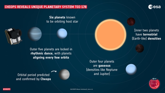
Image: Infographic of the TOI-178 planetary system. Credit: ESA.
But more to the point of the TRAPPIST-1 comparison, whereas the seven planets there show similar densities, implying like compositions, the six worlds around TOI-178 show, in complete contrast to the orderly harmonics of their orbits, a wide range in density. The two inner planets have densities compatible with rocky worlds, while the outer four are gaseous. This is unusual for systems in this kind of complex resonance. No wonder ESA project scientist Kate Isaak is drawn up short:
“It is the first time we observe something like this. [In] the few systems we know with such a harmony, the density of planets steadily decreases as we move away from the star. In the TOI-178 system, a dense, terrestrial planet like Earth appears to be right next to a very fluffy planet with half the density of Neptune followed by one very similar to Neptune.”
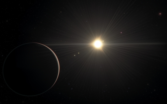
Image: This artist’s impression shows the view from the planet in the TOI-178 system found orbiting furthest from the star. New research by Adrien Leleu and his colleagues with several telescopes, including ESO’s Very Large Telescope, has revealed that the system boasts six exoplanets and that all but the one closest to the star are locked in a rare rhythm as they move in their orbits. But while the orbital motion in this system is in harmony, the physical properties of the planets are more disorderly, with significant variations in density from planet to planet. This contrast challenges astronomers’ understanding of how planets form and evolve. This artist’s impression is based on the known physical parameters for the planets and the star seen. Credit: ESO/L. Calçada/spaceengine.org.
To produce the study, the CHEOPS measurements were enhanced by the addition of data from the TESS mission as well as the ESO spectrograph ESPRESSO, allowing scientists to measure the orbits and sizes of the planets: The orbital periods are 1.91, 3.24, 6.56, 9.96, 15.23, and 20.71 days respectively, while size ranges from 1.1 to 3 times Earth’s radius. It’s interesting to see that the 6th world around TOI-178 was found by extrapolating from the resonance pattern to look for a planet in a 15-day orbit to match the chain. After a short shutdown of CHEOPS observations, additional data were collected, confirming the existence of the 6th world. From the paper:
Careful analysis of the whole system additionally revealed that planets c, d, e, and g were in a Laplace resonance. In order to fit in the resonant chain, the unknown period of the additional planet could have only two values: P = 13.4527 d or P = 15.2318 d…, the latter value being more consistent with the RV data. A fourth CHEOPS visit was therefore scheduled for 3 October, and it detected the transit for the additional planet at a period of 15.231915 day[s]…
Lead author Adrien Leleu (University of Bern, University of Geneva and the National Center of Competence in Research PlanetS) puts the matter this way:
“This result surprised us, as previous observations with the Transiting Exoplanet Survey Satellite (TESS) of NASA pointed toward a three planets system, with two planets orbiting very close together. We therefore observed the system with additional instruments, such as the ground based ESPRESSO spectrograph at the European Southern Observatory (ESO)’s Paranal Observatory in Chile, but the results were inconclusive… After analyzing the data from eleven days of observing the system with CHEOPS, it seemed that there were more planets than we had initially thought.”
The animation below puts the system into motion.
Image: Artist’s animation of the TOI-178 orbits and resonances: This animation shows a representation of the orbits and movements of the planets in the TOI-178 system. The system boasts six exoplanets and all but the one closest to the star are in resonance. This means that there are patterns that repeat themselves rhythmically as the planets go around the star, with some planets aligning every few orbits. In this artist’s animation, the rhythmic movement of the planets around the central star is represented through a musical harmony, created by attributing a note (in the pentatonic scale) to each of the planets in the resonance chain. This note plays when a planet completes either one full orbit or one half orbit; when planets align at these points in their orbits, they ring in resonance. Credit: © ESO / L. Calçada.
Could there be other planets here? The paper points to other possible signals of transiting worlds in the data:
As there is no theoretical reason for the resonant chain to stop at 20.7 days, and the current limit probably comes from the duration of the available photometric and RV datasets, we give in Table 7 the periods that would continue the resonant chain for first-order (q = 1) and second-order (q = 2) MMRs [Mean Motion Resonance chains]… In the TOI-178 system, as well as in similar systems in Laplace resonance, planet pairs are virtually all nearly first-order MMRs. The most likely of the periods shown in Table 7 are therefore the first-order solutions with low k [a reference to the period ratio of the planets, with k being an integer], hence 45.00, 32.35, or 28.36 days; however, additional planets with such periods would not be transiting if they were in the same orbital plane as the others…
If you’re wondering (as I was), TOI-178’s habitable zone should have an inner boundary, according to the authors, at about 0.2 AU, producing a planet with a period of 40 days or so. In other words, other possible planets in the Laplace resonance chain could orbit inside or close to the habitable zone. Those we’ve found so far do not.
The use of resonance in predicting the existence of an exoplanet in such a complex system stands out. The authors call mean-motion resonance chains ‘Rosetta Stones’ of planetary system formation and evolution, and note that such configurations may emerge as protoplanetary disks evolve. But subsequent dissipation of the protoplanetary disk and tidal forces among closely spaced planets can produce instabilities that disrupt the resonance. The result is, as the authors note, that “resonant configurations are not the most common orbital arrangements.”
The paper is Leleu et al., “Six transiting planets and a chain of Laplace resonances in TOI-178,” accepted at Astronomy & Astrophysics (abstract / Preprint).

TRAPPIST-1: Seven Worlds of Similar Compostion
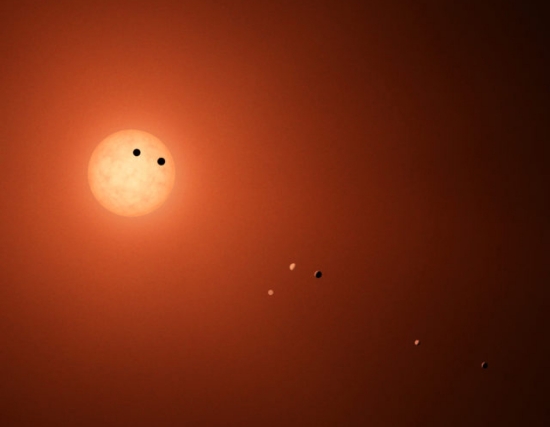
Image: Artist’s depiction of the TRAPPIST-1 star and its seven worlds. Credit: NASA/JPL-Caltech/R. Hurt (IPAC).
As if we needed another indication that the TRAPPIST-1 system is utterly different from our own, consider new work led by Eric Agol (University of Washington), which examines this seven-planet system in terms of the planets’ density. The planets here are all similar in size to Earth. Compare that with the huge range in planetary size we see in our own system. The new work tightens orbital dynamics and calculates their densities, showing they are all about 8 percent less dense than the rocky planets around Sol.
In the paper, the TRAPPIST-1 densities are calculated through analysis of abundant data (over 1,000 hours of observation by Spitzer alone, along with significant contributions from Kepler and ground-based telescopes like TRAPPIST and SPECULOOS). They are refined through computer simulations on planetary orbits, showing a system where planetary composition begs for an explanation.
We’re dealing with a system under intense scrutiny, one about which we have ever-tightening parameters on planetary diameter, mass and density, so we have much to work with. The work pauses briefly to consider a possible eighth planet:
Our mass precisions are predicated on a complete model of the dynamics of the system. We ignore tides and general relativity, which are too small in amplitude to affect our results at the current survey duration and timing precision (Bolmont et al. 2020). Should an eighth planet be lurking at longer orbital periods, which has yet to reveal itself via significant TTVs or transits, this may modify our timing solution and shift the masses slightly. In our timing search for an additional planet, however, we found that such a planet might only cause shifts at the ≈1σ level.
Agol worked with colleagues Zachary Langford and Victoria Meadows at the University of Washington, and an international team including scientists based in Switzerland, France, the UK and Morocco. Says Agol:
“This is one of the most precise characterizations of a set of rocky exoplanets, which gave us high-confidence measurements of their diameters, densities and masses. This is the information we needed to make hypotheses about their composition and understand how these planets differ from the rocky planets in our solar system.”
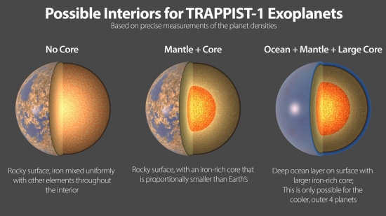
Image: Shown here are three possible interiors of the TRAPPIST-1 exoplanets. The more precisely scientists know the density of a planet, the more they can narrow down the range of possible interiors for that planet. All seven planets have very similar densities, so they likely have a similar compositions. Credit: NASA/JPL-Caltech.
The researchers examine the TRAPPIST-1 planets in terms of the proportion of iron, oxygen, magnesium and silicon thought to make up rocky worlds in any system. The 8 percent difference in density is explicable through several competing hypotheses.
A lower percentage of iron — 21 percent as compared to Earth’s 32 percent — would do the trick, possibly indicating a core with a lower relative mass (most of Earth’s iron is found in its core). Alternatively, planets enriched with oxygen compared to the Earth could produce iron oxide — rust — in abundance, possibly extending to the core (Earth, Mars, Mercury and Venus have cores of unoxidized iron). A combination of both these scenarios is possible, according to Agol, with the TRAPPIST-1 planets having less iron than our system’s rocky worlds but with a larger amount of it being oxidized.
A third possibility is that these planets are enriched with water compared to the Earth. Surfaces covered with water would change a planet’s overall density. This would demand amounts of water totalling 5 percent of the total mass of the four outer planets (by comparison, water makes up less than 0.1 percent of the Earth’s total mass). This would also imply hot, dense atmospheres for the three inner worlds at TRAPPIST-1.
Each hypothesis has consequences in terms of planet formation. Water worlds imply origins beyond the snow line, an environment rich in ice, with the planets subsequently migrating inward toward the host star. Long-term planetary configurations can form from migration, and the stability of TRAPPIST-1’s system has been examined in earlier work. Tightening up the constraints on planetary mass and orbital eccentricity allows the authors to again consider the question. They find that the idea of migration also fits the hypothesis of a fully oxidized planetary core. From the paper:
…the lower measured bulk densities of the TRAPPIST-1 planets relative to Earth-like composition might be explained by core-free interiors (Elkins-Tanton & Seager 2008) in which the oxygen content is high enough such that all iron is oxidized. If the refractory elements (Mg, Fe, Si) follow solar abundances, a fully oxidized interior would contain about 38.2 wt% of oxygen, which lies between the value for Earth (29.7 wt%) and CI chondrites (45.9 wt%). Such an interior scenario can easily describe the observed bulk densities…, and this may bolster the long-range migration scenario in which the planets formed in a highly oxidizing environment that enabled the iron to remain in the mantle even after migration.
One thing that would drive this work further is more information about the composition of the M8 red dwarf that hosts the planetary system. The authors point out that measurements of the Mg/Fe and Fe/Si ratios would affect the interpretation of their results on planetary cores and mantle composition.
And as we see so often in such work, a functioning James Webb Space Telescope is pointed to as a possibility for producing even more precise constraints on system dynamics and planetary bulk densities, which would aid in choosing among the competing hypotheses for composition. For all of this, the TRAPPIST-1 system is an ideal testing ground, as co-author Caroline Dorn (University of Zurich) notes:
“The night sky is full of planets, and it is only within the last 30 years that we have been able to begin to unravel their mysteries. The TRAPPIST-1 system is fascinating because around this unique star we can learn about the diversity of rocky planets within a single system. And we can also learn more about a planet by studying its neighbours, so this system is perfect for that.”
The paper is Agol et al., “Refining the Transit-timing and Photometric Analysis of TRAPPIST-1: Masses, Radii, Densities, Dynamics, and Ephemerides,” Planetary Science Journal Vol. 2, No. 1 (22 January 2021). Full text.
Was the Wow! Signal Due to Power Beaming Leakage?
The Wow! signal has a storied history in the SETI community, a one-off detection at the Ohio State ‘Big Ear’ observatory in 1977 that Jim Benford, among others, considers the most interesting candidate signal ever received. A plasma physicist and CEO of Microwave Sciences, Benford returns to Centauri Dreams today with a closer look at the signal and its striking characteristics, which admit to a variety of explanations, though only one that the author believes fits all the parameters. A second reception of the Wow! might tell us a great deal, but is such an event likely? So far all repeat observations have failed and, as Benford points out, there may be reason to assume they must. The essay below is a shorter version of the paper Jim has submitted to Astrobiology.
by James Benford

In 1977 the Big Ear radio telescope (Ohio State University Radio Telescope) recorded the famous Wow! Signal, which is the most serious contender for artificial interstellar radiation. It is called the ‘Wow!’ Signal. It has never been seen again. Its origin and nature remain a total mystery.
I offer an alternative explanation for it: The Wow! could have been leakage from an interstellar power beam. I propose that this class of radiation, which is not widely understood, can explain the observed features of the Wow! signal.
The Three Wow! Parameters
The Wow! signal has 3 prominent parameters: the power density received, the signal’s duration and its frequency [1].
Power Density: The Wow! signal was very strong, the strongest they ever recorded in the seven-year Ohio State SETI Survey. The shape is shown in the Figure.
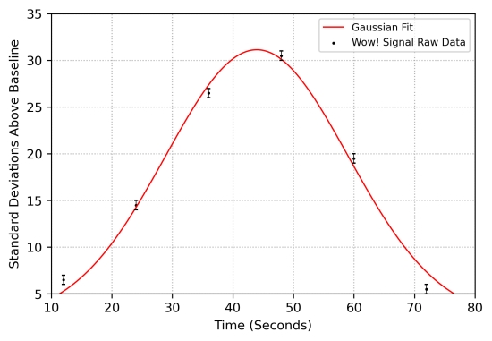
Figure: The Wow! Signal. The peak is 32 times the signal to noise ratio of the observations. Courtesy of Sam Morrell.
Duration: The Big Ear was fixed in orientation, so rotated with the Earth. From Gray [1]: “The amount of time it took the Wow! to pass through the antenna’s beam closely matches the expected transit time for celestial sources. Sources fixed amid the stars should take about 36 seconds to transit the sensitive middle half of the beam, the full-width-half-max. The Wow! signal took about 38 seconds”.
So we don’t know how long the signal lasted, just that it was on as the antenna rotated past.
Frequency: The Wow! Signal was at 1.42 GHz. The 1.4-1.427 GHz band is protected internationally, meaning, as John Kraus, designer and director at the Big Ear, says in a letter to Carl Sagan , “all emissions are prohibited” [2]. The band was set aside to allow radio astronomy of the H 1 line, the hyperfine transition of neutral hydrogen (1.420 GHz), which is of great astronomical interest for imaging atomic hydrogen in interstellar space. Consequently, this part of the L-band is a protected radio astronomy allocation all over the world. Therefore the Wow! couldn’t be a transmission from Earth satellites or aircraft.
The Fourth Wow! Parameter
There is a fourth parameter, although it has not received attention: the Revisit Time. This is the interval until the signal is seen again. If ET were rastering their beam across the sky, the beam would be seen to repeat later. Searches have been conducted from the META array at Oak Ridge, the Green Bank National Radio Astronomy Observatory in West Virginia and the Tasmanian Mount Pleasant Radio Observatory in Australia [3, 4].
Recent extensive observations on the Allen Array by Gerry Harp, Robert Gray and colleagues, which used the 42 dishes of the ATA as an interferometer, monitored the entire 1.5 degree field of view for 100 hours. They did not see the Wow! and summarized [5]: “As for the possibility that the Wow! signal is a repetitive transient, our observations rule out almost all periods under 40 hours, which covers many repetitive scenarios such as rotating planets or blinking beacons with periods comparable to a terrestrial day and several times longer. Our extended observations cannot rule out scenarios such as occasional targeted transmissions with repetition rates of many days or varying repetition rates.”
The Wow! observation has never recurred. I take this absence as a clue to its origin.
Power Beaming and the Wow! Signal
The most observable leakage radiation from an advanced civilization may well be from the use of power beaming to accelerate spacecraft and transfer energy. Power beams are now more credible because we’re building our own: The Starshot project plans launching probes to nearby stars in this century, making power beaming a credible source concept [6]. And power beaming is being developed for military applications, where it is termed ‘directed energy’ [7]. See reference 8 for a review of power beaming concept studies.
Applications suggested for power beaming are:
- launching spacecraft to orbit,
- raising satellites to a higher orbit,
- interplanetary space-to-space transfers of cargo or passengers,
- beam-driven launch of interstellar probes,
- beam-driven starships.
Leakage of the beam around the sides of the vehicle being accelerated would be observable at great range because of the highly directed high power. The spilled energy can be reduced to less than half, but that is not the cost optimum. Spillage losses of more than half are typical of Starshot calculations, for reasons of economics and performance that will apply to other civilizations [6].
For power beam missions involving changing orbits of spacecraft, the first three applications on the above list, an important quantity is the slew rate, the rate at which the beam propelling the spacecraft sweeps to direct it toward its orbit [8]. A review of representative parameters for applications of power beaming shows that, for orbit-related missions, the slew rates are high, so the observation time of the beam leakage is too short, ≲ 1 second. So the orbit-related applications cannot explain the Wow! But interstellar probes and starships have small slew rate, so are the best candidates.
Power Beaming Examples
In beaming of power, the power density S at range R is determined by W, the effective isotropic radiated power (EIRP), which is the product of radiated peak power P and aperture gain G [8]. Since we know the power density of the Wow! received and its frequency, we can calculate both the range to the source of Wow! and the power needed at a given range.
For example, if the Wow! source had the EIRP of Arecibo, it would have to be at range < 2 light-years, so it must be far more powerful.
Bob Forward’s ultralight microwave-propelled Starwisp, a 1-kg sail reaching 0.1 c, would be at a range of ~ a million light-years, so from extra-galactic distances [9].
An interstellar precursor probe described by Benford and Matloff for 100 km/sec = 0.03% c would be at range 116 light-years, a nearby star [10].
We can also assume a distance, then calculate the EIRP that would be required. First, choose 2000 light-years for the distance to the Wow! source. (Maccone estimates that the mean distance to a communicative civilization is ~2,000 light-years away [11]). Then choose an aperture diameter of 3 km. (Starshot envisions a ~3-km diameter laser array to drive its interstellar probe.) The required beam power is 11 GW. This is similar to Starshot, with ~ 11 GW.
From these examples, it is credible that the Wow! signal was leakage from launch of an interstellar probe.
Will we see it again? Probably not
Probably not if it was due to power beaming. With a launch driven by an intense beam, to arrive years later at a neighboring stellar system, the starship would be launched toward where the stellar system will be when the starship arrives. The ratio of the distance the star would move to the beam spot size is given by vs/(vss Δθ), where vs is the average velocity of the star relative to stars on our stellar neighborhood, typically 20 km/sec, and vss is the starship velocity, Δθ the angular beamwidth. For the starship concepts proposed, that ratio varies from 104 to 107 [8].
The angle of the radiated beam with respect to the light path between the two stars is larger than the width of the beam. Thus, the beam is generally not observable from the target planetary system. If the Wow! was driving a probe to a star, that star was at that time far from the direction of the beam. Earth could accidentally receive the leakage from the beam, since stars move relative to each other. So leakage radiation from star probe launches using the Wow! beam will not be seen again from Earth. This fits the non-observations to date.
Comparison of Explanations for the Wow! Signal
There are three suggested explanations for the Wow!: either spurious emissions from Earth, an interstellar communication or leakage from a power beam. Here is a brief summary of the evidence for and against each explanation:
Arguments for power beaming leakage as a cause:
- The power beaming explanation for the Wow! accounts for all four of the Wow! parameters: the power density received, the duration of the signal, its frequency, and the reason why the Wow! has not occurred again. The Wow! power beam leakage hypothesis gets stronger the longer that listening for the Wow! to recur doesn’t observe it repeat.
- Power beams are now more credible because we’re building our own: the Starshot project plans launching probes to nearby stars in this century. The technology required for the Beamers for such interstellar probe launches are within our grasp.
Arguments against ET communication as a cause:
- The theory that the Wow! Signal was an interstellar communication predicts that it will recur. It fits within the overall SETI strategy, which looks for deliberate beaming of messages to us from ETI. But the long series of the subsequent non-observations of the Wow! shows that the SETI messaging hypothesis is gradually being falsified by being tested.
Arguments against radio frequency interference (RFI) as a cause:
- The Wow! Signal was at 1.42 GHz. The band from 1.4 to 1.427 GHz is protected internationally, meaning, all emissions are prohibited [2]. Therefore it is very doubtful that the Wow! Was a transmission from Earth satellites or aircraft because they are forbidden to transmit in this band. Secret satellites would avoid it because they would be detected by radio astronomers. (Emissions in this band are sometimes detected, but at very low levels. These are likely due to intermodulation products, which are nonlinear effects in electronics.)
- Aircraft would be unlikely to remain static in the sky. Spacecraft would pass through the beam much faster. To match that lack of angular motion, an Earth satellite would have to be millions of kilometers distant, out far beyond the Moon.
- Ohio had good RFI rejection because what was recorded was the difference between two offset beams, so a local signal appearing in both horns simultaneously would cancel. This was frequently verified.
- The possibility that the signal was a harmonic or sub-harmonic of a local signal is countered by Ohio State having monitored the 21 cm band for many years, would have noticed a local interfering signal.
- A deliberate hoax? This lacks credibility, as hoaxes are a practical joke, which succeed if they are later revealed. Then why keep it secret for decades?
Conclusion and Implications
I’ve looked at the various power beaming applications and found that credible ones are low mass interstellar probes such as Starwisp and Starshot. This does not mean that the orbit-changing power-beaming applications cannot be seen.
The power beaming explanation for the Wow! accounts for all four of the Wow! parameters. This includes the absence of any later observation, for it has not been seen since, despite the several attempts to repeat observing it. This allows a prediction: the Wow! signal will not be seen again.
If one accepts the possibility that Wow! was power beam leakage, several lines of action should be followed for the future of SETI:
- Such interstellar power beams would be visible over large interstellar distances. All-sky surveys in both the microwave and laser could detect more power beam leakages. Instruments with large instantaneous field of view could detect infrequent transitory leakage signals. Ultimately, we should have a full-sky capability for both hemispheres.
- Because ET would understand that its beam leakage could be observed, there may well be modulations on the beam to communicate to any inadvertent listener. This would add little additional energy or cost for ET. Therefore all-sky surveys should have sufficient electronics to capture messaging embedded on the beam. Extraterrestrial intelligences would know their power beams could be observed. That message may use optimized power-efficient designs such as spread spectrum and energy minimization [12, 13].
On the other hand, if one thinks that the Wow! signal was an attempt to communicate, one should follow up on a possibility that is not been explored: If with Wow! we inadvertently intercepted a radio link between one star and another, we should look in the opposite direction to see if signals are transmitting toward the Wow! direction. To my knowledge this has not been explored.
References
1. R. H. Gray, The Elusive Wow!, Palmer Square Press, 2012.
2. J. D. Kraus, “The Tantalizing “Wow!” Signal”, letter to Carl Sagan, NRAO Archives, accessed December 3, 2020, https://www.nrao.edu/archives/items/show/3684, 1994.
3. R. H. Gray, “Intermittent Signals and Planetary Days in SETI”, Int. J. Astrobiology, https://doi.org/10.1017/S1473550420000038
4. R. H. Gray, A Search For Periodic Emissions At The Wow! Locale”, Astrophysical Journal, 578:967-971, 2002.
5. G. Harp et al., “An ATA Search for a Repetition of the Wow! Signal”, Astrophysical Journal 160:162, 2020.
6. K. Parkin, “The Breakthrough Starshot System Model”, Acta Astronautica 152, 370, 2018.
7. J. Benford, J. Swegle and E. Schamiloglu, High Power Microwaves, 3rd Ed., Taylor & Francis, Boca Raton, FL 2016.
8. J. Benford and D. Benford, “Power Beaming Leakage Radiation as a SETI Observable”, Astrophysical Journal 101 825, 2016.
9. R. L. Forward, “Starwisp: An Ultralight Interstellar Probe,” J. Spacecraft and Rockets, 22 345-350 1985.
10. J. Benford and G. Matloff, Intermediate Beamers for Starshot”, JBIS 72, 51, 2019.
11. C. Maccone, “The Statistical Drake Equation”, Acta Astronautica 67, 1366, 2010.
12. D. Messerschmitt, “The case for spread spectrum”, Acta Astronautica, 81, 227, 2012.
13. D. Messerschmitt, 2015, ‘Design for minimum energy in interstellar communication”, Acta Astronautica, 107, 20-39, 2015.
Propulsion for Satellite ‘Constellations’
A French company called Exotrail has been working on electric propulsion systems for small spacecraft down to the CubeSat level. As presented last week at the 13th European Space Conference in Brussels, the ExoMG Hall-effect electric propulsion system was flown in a demonstration orbital mission in November, launched to low-Earth orbit by a PSLV (Polar Satellite Launch Vehicle) rocket. A brief nod to the PSLV: These launch vehicles were developed by the Indian Space Research Organisation (ISRO), and are being used for rideshare launch services for small satellites. Among their most notable payloads have been the Indian lunar probe Chandrayaan-1, and the Mars Orbiter Mission called Mangalyaan.
Hall-effect thrusters (HET) trap electrons emitted by a cathode in a magnetic field, ionizing a propellant to create a plasma that can be accelerated via an electric field. The technology has been in use in large satellites for many years because of its high thrust-to-power ratio.
What catches my eye about ExoMG is its size, about that of a 2-liter bottle of soda as opposed to conventional Hall-effect thrusters that weigh in at refrigerator size and demand kilowatts of power. The Exotrail thruster, which was successfully fired during the November mission, runs on about 50 watts of power, and appears to be a propulsion system that can adapt to satellites in the range of 10 to 250 kg. Collision avoidance and deorbiting for satellites in the CubeSat range as well as flexible orbital operations become feasible with this technology.

Image: Satellite using Exotrail technology undergoing testing. Credit: Exotrail.
The company is calling ExoMG “the first ever Hall-effect thruster operating on a sub-100kg spacecraft,” and points to four missions slated to fly with the technology in 2021. I’m interested in how the diminutive thruster can be employed in constellations of satellites. We already rely on satellites working together as a system — GPS is a classic example. The needs of navigation and communication force the issue. Think Iridium and Globalstar in terms of telephony, or the Russian Molniya military and communications satellites. The list could be easily extended.
So what we have evolving is a set of constellation technologies with immediate application to satellites in low-Earth orbit. Exotrail talks about “high coverage telecommunication constellations or high revisit rate earth observation constellations at 600-2000km altitude,” enabled by orbit-raising via the new thrusters as well as necessary de-orbiting capabilities, but we should be looking as well at the controlling software and thinking in longer timeframes. Satellites working together is the theme.
Increasing miniaturization coupled with artificial intelligence and next-generation electric thrusters can be enablers for planetary probes flying in swarm formation in the outer system, perhaps using sail technologies as the primary propulsion to get them there. The one-size fits all purposes mission begins to give way to a fleet approach, tiny probes networking their data as they operate at targets as interesting as Neptune and Pluto. It’s also worth noting that the entire Breakthrough Starshot concept calls for not one but an armada of small sails in interstellar space, offering a hedge against catastrophic failure of any one craft, and conceivably drawing on swarm technologies that could facilitate data gathering and return.
So I keep an eye on near-term technologies that explore this space of miniaturization, efficient orbital adjustment and constellation operations. It will be intriguing to see how Exotrail’s operational software (called ExoOPS) deals with the interactions of such constellations. Likewise interesting is last fall’s firing of the European Space Agency’s Helicon Plasma Thruster, which ESA presents as a “compact, electrodeless and low voltage design” optimized for propulsion in small satellites, including “maintaining the formation of large orbital constellations.”
The HPT achieved its first test ignition back in 2015 at ESA’s Propulsion Laboratory in the Netherlands, and has been under development in terms of improved levels of ionization and acceleration efficiency ever since, using high-power radio frequency waves, as opposed to the application of an electrical current, to render propellant into a plasma for acceleration.
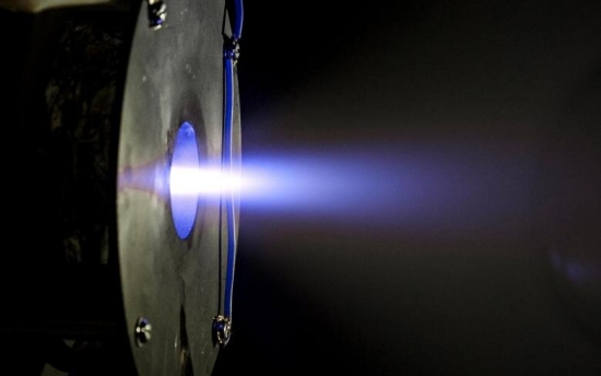
Image: A test firing of Europe’s Helicon Plasma Thruster, developed with ESA by SENER and the Universidad Carlos III’s Plasma & Space Propulsion Team (EP2-UC3M) in Spain. This compact, electrodeless and low voltage design is ideal for the propulsion of small satellites, including maintaining the formation of large orbital constellations. Credit: SENER.
Where will constellation and formation flying in Earth orbit take us as we adapt them for environments further out? Will we one day see deep space swarms of Cubesat-sized (and smaller) craft exploring the outer planets?
TOI-1259A: Implications of a White Dwarf Companion
TESS, our Transiting Exoplanet Survey Satellite, continues to roll up interesting planet candidates, with over 2450 TESS Objects of Interest (TOI) thus far identified. The one that catches my eye this morning showed up in the lightcurve of TOI-1259A, a K-dwarf some 385 light years away. The planet designated TOI-1259Ab is Jupiter-sized but some 56 percent less massive, with a 3.48 day orbit at 0.04 AU, and an equilibrium temperature of 963 K.
This system gets interesting, though, not so much for the planet but the other star, a white dwarf (TOI-1259B) in a wide orbit at 1648 AU from the K-dwarf. A team of astronomers led by David Martin (Ohio State University) finds an effective temperature of 6300 K, a radius of 0.013 solar radii and a mass of 0.56 solar masses, a set of characteristics that allow the team to estimate that the system is just over 4 billion years old.
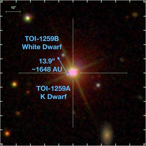
Image: SDSS image of the planet host TOI-1259A and its bound white dwarf companion TOI-1259B. Credit: Martin et al., 2021.
Let’s home in on the issue of white dwarfs, for they force a significant question: How does the evolution of a star affect the evolution of the planetary system around it? The system containing TOI-1259Ab may prove useful in helping us understand the processes at work.
But first, what about white dwarfs themselves? A star like the Sun will expand into a red giant perhaps five billion years from now, ultimately leaving a white dwarf remnant, with whatever planetary survivors still intact left transformed by the process.
So it’s not surprising that about 50 percent of the white dwarfs studied show atmospheres polluted by heavy elements. That would be an indication of material from the surrounding system accreting onto the white dwarf. Still noteworthy, though, is the fact that you would expect such heavy elements to settle out in the presence of the white dwarf’s high gravity. The process of accretion must, then, be relatively common, allowing the stellar atmosphere to be constantly replenished.
White dwarfs produce their own set of challenges when it comes to exoplanet discovery. Finding planets around them is relatively rare. From the paper on the TOI-1259Ab work, I learned that these stars show a lack of the kind of sharp spectral features that would allow precise characterization using radial velocity methods. The push and pull of orbiting worlds is less evident than it would be around other classes of star.
That seems to throw us back on transit methods, something both Kepler and TESS turned into an art, but here we’re dealing with the problem that white dwarfs have a small radius. They’re roughly the size of the Earth, which means that transit probabilities are reduced and so are transit durations. Moreover, according to Martin et al., white dwarfs are faint enough that their light curves are noisy, a problem for astrometric methods — think Gaia — as well.
So while we’ve found atmospheric pollutants at these stars, and have tagged transits of planetary debris, the first confirmed planet orbiting a white dwarf wasn’t found until recently (for more on WD 1856+534, see On White Dwarf Planets as Biosignature Targets).
But back to TOI-1259Ab, which is not a white dwarf planet, but a tightly orbiting Jupiter-sized planet around a K-dwarf. Here the white dwarf is a distant but definitely bound second star. It turns out that even systems with planets and white dwarf companions are rare, as the paper notes:
Only a few bona fide planets have been discovered with degenerate outer companions (Table 2), the first being Gliese-86b (Queloz et al. 2000; Els et al. 2001; Lagrange et al. 2006). Mugrauer (2019) found 204 binary companions in a sample of roughly 1300 exoplanet hosts, of which eight of the companions were white dwarfs. Mugrauer & Michel (2020) found five white dwarf companions to TESS Objects of Interest, including TOI-1259, but without radial velocity data to confirm the TOIs as planets. Some of these planets were also in the El-Badry & Rix (2018) catalogue.
Stellar systems that include white dwarfs have much to teach us, and in the case of TOI-1259Ab, we have a world that has now been confirmed through radial velocity follow-up, and a white dwarf that influenced it. Driving this research forward will be the question of how systems with a degenerate outer companion object evolve, for there are implications here for planetary dynamics. This system should be an interesting target for the James Webb Space Telescope. Consider: The transit depth is 2.7 percent on the K-dwarf host star, which is 0.71 percent of the Sun’s radius. Moreover, its location places the system near the TESS and JWST continuous viewing zones.
The authors believe that the white dwarf in this system is far enough from the K-dwarf that it would not affect the formation of planets, but go on to point out that while it was on the main sequence, it progenitor star would have been both more massive and also closer, which would have made it a factor in orbital dynamics for TOI-1259Ab. The planet’s tight orbit may thus be at least partially the result of migration forced by the now degenerate white dwarf companion.
On the matter of stellar age, it’s worth noting that white dwarfs cool steadily as they age, which helps astronomers constrain the age of the star and the system around it using its temperature and luminosity. Let me quote the paper on this, because star age is so tricky to determine for other stellar types:
If the WD’s mass is known, the initial mass of its progenitor star can be inferred through the initial-final mass relation (IFMR), and this initial mass constrains the pre-WD age of the WD progenitor. Therefore if we have a well-constrained distance to the WD then its total age, i.e. the sum of its main sequence lifetime and its cooling age, can be robustly measured from its spectral energy distribution (SED). Under the reasonable ansatz that the WD and K dwarf formed at the same time, we can then measure the total system age from the WD.
Another useful insight offered by white dwarfs, the study of which may help us explain unusual system architectures like this one, as well as informing us on outcomes as stars and their companions are transformed over time.
The paper is Martin et al., “TOI-1259Ab – a gas giant planet with 2.7% deep transits and a bound white dwarf companion,” submitted to Monthly Notices of the Royal Astronomical Society (preprint).
Recovering a Triple Star Planet with New Data
The Kepler mission produced so much data — 2394 exoplanets, 2366 candidates by the end of spacecraft operations in 2018 — that we might forget how quickly all this came about. The first Kepler results started being announced in 2010. One of these, the second candidate to emerge, was KOI-5Ab, which was a tough pick in the early going given its position within a triple star system. An ambiguous detection, it was soon left behind, its status uncertain, as the numbers of more definitive candidates swelled. Caltech’s David Ciardi, who discussed this elusive system at the recent virtual meeting of the American Astronomical Society, says this about it:
“KOI-5Ab got abandoned because it was complicated, and we had thousands of candidates. There were easier pickings than KOI-5Ab, and we were learning something new from Kepler every day, so that KOI-5 was mostly forgotten.”
Ciardi, who is chief scientist at NASA’s Exoplanet Science Institute, has now pulled KOI-5Ab back to vibrant life. Almost certainly a gas giant, the planet orbits one of three stars in the system in a misaligned orbit that calls into question the nature of its formation. Making original confirmation of the planet difficult was the inability to completely distinguish it from the possible effects of the other two stars in the system. Untangling the question would involve TESS data. The object appears in TESS terminology as TOI-1241b, showing a five-day orbit that matches the Kepler result.
Confirming such a candidate calls for more than a single backup asset on the ground. Working with colleagues in the California Planet Search, Ciardi used Keck data, as well as observations from Caltech’s Palomar Observatory near San Diego and Gemini North in Hawaii, though the scientist credits TESS as the motivation for re-visiting the object. We learn that KOI-5Ab orbits Star A, whose companion, Star B, is in a tight 30 year orbit with A. The third star orbits A and B every 400 years. Have a look at the image below to see the orbital dance.
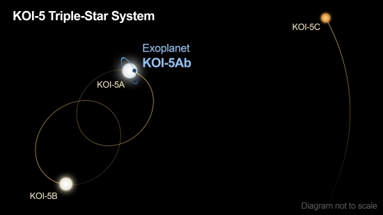
Image: The KOI-5 star system consists of three stars, labeled A, B, and C in this diagram. Star A and B orbit each other every 30 years. Star C orbits stars A and B every 400 years. The system hosts one known planet, called KOI-5Ab, which was discovered and characterized using data from NASA’s Kepler and TESS (Transiting Exoplanet Survey Satellite) missions, as well as ground-based telescopes. KOI-5Ab is about half the mass of Saturn and orbits star A roughly every five days. Its orbit is titled 50 degrees relative to the plane of stars A and B. Astronomers suspect that this misaligned orbit was caused by star B, which gravitationally kicked the planet during its development, skewing its orbit and causing it to migrate inward. Credit: Caltech/R. Hurt (IPAC).
The orbital mechanics in play as planets formed from a primordial disk could account for the misalignment, given the gravitational influence of the second star, causing the planet to migrate inward as well as skewing its inclination. There are similar cases of misaligned orbits — particular GW Orionis — offering evidence of distortions caused by multiple star system evolution.
“We don’t know of many planets that exist in triple-star systems, and this one is extra special because its orbit is skewed,” adds Ciardi. “We still have a lot of questions about how and when planets can form in multiple-star systems and how their properties compare to planets in single-star systems. By studying this system in greater detail, perhaps we can gain insight into how the universe makes planets.”
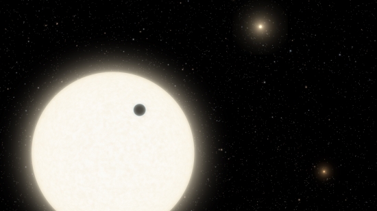
Image: This artist’s concept shows the planet KOI-5Ab transiting across the face of a sun-like star, which is part of a triple-star system located 1,800 light-years away in the constellation Cygnus. Credit: Caltech/R. Hurt (IPAC).

Follow with RSS or E-Mail
