Centauri Dreams
Imagining and Planning Interstellar Exploration
Impact in the Outer System
We looked recently at Voyager 2’s flyby of Uranus, via a new paper that examined the craft’s magnetometer data to draw out information about the planet’s magnetic environment. Science fiction author Stanley Weinbaum, author of the highly influential “A Martian Odyssey” in 1935, christened Uranus ‘The Planet of Doubt’ in a short story of the same name. Weinbaum couldn’t have known about the world’s magnetic field axis, which we’ve learned is tilted 60 degrees away from its spin axis. The latter itself is 98 degrees off its orbital plane. Doubtful planet indeed.
Here we have a world that is spinning on its side, one that demands answers as to how it got that way. A giant impact at some point in its history is a natural assumption, but how do we explain the fact that the Uranian moons as well as the planet’s ring system all show the same 98 degree orbital tilt as their parent? Back in 2011, a team led by Alessandro Morbidelli (Observatoire de la Cote d’Azur) ran a variety of simulations to test impact scenarios and discovered that a sufficiently early impact could have reformed the entire protoplanetary disk, leading to its 27 moons being in the position we see today. See the Centauri Dreams post A New Slant on the Planet of Doubt for more on the Morbidelli et al. paper.
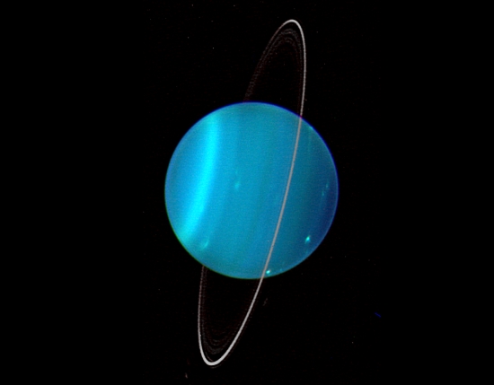
Image: Uranus is uniquely tipped over among the planets in our Solar System. Uranus’ moons and rings are also orientated this way, suggesting they formed during a cataclysmic impact which tipped it over early in its history. Credit: Lawrence Sromovsky, University of Wisconsin-Madison/W.W. Keck Observatory/NASA.
Now we have another look at the problem, this from a team led by Shigeru Ida (Earth-Life Science Institute, Tokyo Institute of Technology). The key to this new paper is the understanding that while impacts would have been more common in the early Solar System than now, the outer planets would have experienced impacts that were different in result than those in the inner system. A rocky Mars-sized object might smack into a rocky Earth to create our Moon, but collisions between two icy objects have different results in the outer Solar System.
Out here, we’re dealing with planets with an abundance of volatiles, elements that would be gases or liquids in the warmer regions of the inner system, but are frozen at large distances from the Sun. The temperature needed to vaporize water ice is low, and the team assumes, reasonably, that both Uranus and its impactor were dominated by ices. Thus an impact early in the formation history of Uranus would have vaporized this ice, with leftover materials remaining gaseous and becoming incorporated primarily into the forming planet. Ida’s computer modeling shows that such impacts produce not one or two large moons but a number of small ones.
The inclination of both ring and moon system at Uranus makes it clear that the impact was early and formative for the entire Uranian system. Bear in mind that the ratio of the planet’s mass to its moons is larger than the ratio of Earth’s mass to its Moon by a factor of more than one hundred. Working with substantial water vapor mass loss, the researchers’ simulation reproduces the observed mass-orbit configuration of the Uranian satellites by incorporating the predicted distribution of ices as they re-condense. The results parallel the system we see today, indicating it is the result of the evolution of this volatile-laden impact-generated disk.
The authors contrast this with the giant impact model for Earth’s Moon, arguing that about half of the solid or liquid disk created by the strike was integrated into the Moon. The difference is the high condensation temperature at Earth’s orbital distances, meaning that the rocky and liquid material of the Earth-Moon impact would have solidified quickly, allowing the Moon to collect a significant amount of the debris created by the collision due to its gravity shortly after impact.
The work may have applications in other stellar systems. From the paper:
We have shown that the current Uranian major satellites are beautifully reproduced by the derived analytical formulas based on viscous spreading and cooling of the disk generated by an impact that is constrained by the spin period and the tilted spin, independent of details of the initial disk parameters. Although we have focused on Uranus, the model here provides a general scenario for satellite formation around ice giants with the scaling by the mass and the physical radius of a central planet, which is totally different from satellite formation scenarios around terrestrial planets and gas giants. It could also be applied for the inner region of Neptune’s satellite system, where we can neglect the effect of Triton that may have been captured. Observations suggest that many of [the] discovered super-Earths in exoplanetary systems may consist of abundant water ice, even in close-in (warm) orbits. The model here may also give a lot of insights into possible icy satellites of super-Earths.
The paper is Shigeru Ida et al., “Uranian satellite formation by evolution of a water vapour disk generated by a giant impact,” Nature Astronomy 30 March 2020 (abstract / preprint).

The Interstellar Ramjet at 60
The interstellar ramjet conceived by Robert Bussard may have launched more physics careers than any other propulsion concept. Numerous scientists over the years have told me how captivated they were with Poul Anderson’s treatment of the idea in his novel Tau Zero. Al Jackson takes a look at Bussard’s concept in today’s essay, referencing its subsequent treatment in the literature and adding a few anecdotes about Bussard himself. The original paper was submitted on February 1, 1960 to Astronautica Acta, then edited by Theodore von Kármán (a ‘tough judge,’ Al notes) and published later that spring. Although the ramjet faces numerous engineering issues, its ability to resolve the mass-ratio problem in interstellar flight makes it certain to receive continued scrutiny.
by A. A. Jackson
Writers of science fiction prose noticed the difference between interplanetary flight and interstellar flight earlier than anyone. Various fictional methods of faster-than-light (FTL) were invented in the 1930s, John Campbell even inventing the term ‘warp drive’. Asimov’s Galactic Empire is only facilitated by FTL ‘jump-drives’. Slower than light interstellar travel made an appearance in Goddard and Tsiolkovsky’s writings in the form of ‘generation ships’, usually called ‘worldships’ now.
As far as I know, the first engineer to look at the very basic physics — quantitative calculations — of relativistic interstellar flight was Robert Esnault-Pelterie; he made relativistic calculations before 1920 that were published in his book L’Astronautique (1930). The first derivation of the relativistic rocket equation occurs in Esnault-Pelterie’s writings. This was long before Ackeret (J. Ackeret, “Zur Theorie der Raketen,” Helvetica Physica Acta 19, p.103, 1946). The classical mass ratio rocket equation of Tsiolkovsky showed the difficulty of space travel. The relativistic rocket equation showed that interstellar flight was even more difficult.
Eugen Sänger, who had been interested in interstellar flight in the 1930s, addressed the interstellar mass ratio problem in 1953 with a paper on photon rockets, “Zur Theorie der Photonenraketen” (Vortrag auf dem 4. Internationalen Astronautischen Kongreß in Zürich 1953). Sänger, more than almost anyone before him, studied the hard physics of antimatter rockets and relativistic rocket mechanics. Using the most energetic energy source, antimatter, would require tons of it in a conventional rocket. There was sore need of a better method.
Bussard
Robert W Bussard was a rangy man who looked like he walked the halls of power. I had dinner with him at a San Francisco section of the American Institute of Aeronautics and Astronautics meeting in 1979. We had invited Poul Anderson, author of Tau Zero; Anderson and Bussard had never met. Over dinner Bussard told me he started working on nuclear propulsion at Los Alamos in 1955, and that he and R. DeLauer wrote the first monograph on atomic powered rockets in 1959 [1]. He also said he had been looking at work at Lawrence Radiation Laboratory in 1959.
Bussard told me he had always been interested in interstellar flight. One day at breakfast at Los Alamos he got a tortilla rolled up with scrambled egg in it. That cylinder made him think of a fusion ram starship! I have to wonder if that story is true, for had he been looking at Livermore’s lab papers he probably saw Project Pluto, the nuclear powered atmospheric ramjet.
Bussard sat down in 1959 and wrote the paper “Galactic matter and interstellar flight,” published in Astronautica Acta in 1960. This paper is thoroughly technical; Bussard summarizes Ackeret, Sänger and Les Shepherd’s studies of interstellar flight [2]. Sänger had shown that even using antimatter one still had a mass ratio problem with a conventional rocket. Bussard then presents an amazing new concept that solved the mass ratio problem [3]. He notes that one can scoop interstellar hydrogen and fuse it to produce a propulsion system.
The treatment is rigorously special relativistic; using conservation of energy and momentum he derives the equations of motion of an interstellar ramjet. He accounts for the energy production and propulsion efficiency of the vehicle in general terms. He uses the most energetic fusion mechanism, the proton-proton fusion reaction which converts .0071 of the rest mass of collected protons to energy. Bussard derives the property that the ramjet will need to be boosted to an initial speed.
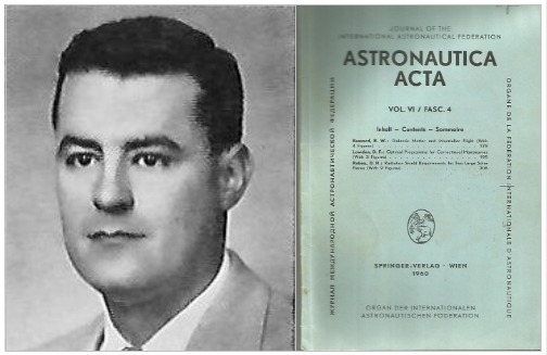
Image: Robert Bussard in 1959 with his Astronutica Acta issue.
Bussard discusses the engineering physics problems; the difficulty of using the p-p chain is enormous. He notes that interstellar hydrogen can be unevenly distributed, there being rich and rarefied regions. He gives a simplified model for scooping and sometimes it is missed that he mentions magnetic fields as a ‘collector’. Bussard also notes both radiation losses and radiation hazards during the operation of the ramjet.
Sagan
The Bussard Ramjet got a boost in 1963 when Carl Sagan noted that there was a solution to the mass ratio problem for interstellar flight [4]. Sagan summarized this paper in Intelligent Life in the Universe in 1966 [5], probably the best popularization of the Ramjet. Sagan also noted that ships accelerating at one gravity could circumnavigate the universe, ship proper time, in about 50 years. He references Sänger in the paper version [4] and the calculation of the mechanics of a 1g starship. As far as I know, the 1957 paper of Sänger [6] is the first exposition of a constant acceleration starship and the consequences of time dilation when extreme interstellar distances are traveled. Bussard mentioned, very briefly, a magnetic field as a scoop, but Sagan describes such a collector in a more elaborated though qualitative way.
Fishback
John Ford Fishback published his MIT bachelor’s thesis in Astronautica Acta in 1969 [7]; this was supervised by Philip Morrison. Morrison and Cocconi were the fathers of radio SETI. Morrison seems to have taken an interest in Sagan’s mention of Bussard’s ramjet — I’m not sure if it was Morrison or Fishback who suggested the study. The paper is a remarkable marshalling of electrodynamics, charged particle motion, plasma physics, the physics of materials and special relativity.
Fishback constructs a model for the magnetic scoop field taking into account the fraction of hydrogen ingested and reflected. Using conservation laws, he derives the most detailed equations of motion accounting for mass and radiation losses that had been published anywhere. In the scooping process, Fishback examines the statistical distribution of gas in the galaxy and derives a relativistic expression for ship proper acceleration with ‘drag’. An important consequence, expressed for the first time, is the mechanical stress on the scoop field magnets. He derived an upper limit on the maximum Lorentz factor that can be obtained as a ramjet accelerates at 1 g for a long time due to stress on the source of the scoop field.
[For more on Fishback, see Al’s John Ford Fishback and the Leonora Christine from 2016, with further thoughts by Greg Benford.]
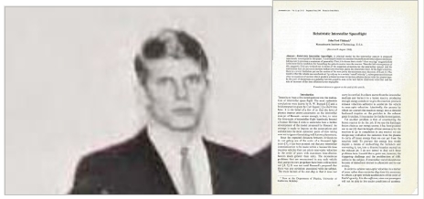
Image: John Ford Fishback in 1967 and first page of his paper in Astronautica Acta. Sadly, Fishback would take his own life in 1970 at the age of 23.
Martin
In 1971 [8] and 1973 [9] Tony Martin reviewed Fishback’s paper, making useful clarifying observations. Martin provides details of calculation that Fishback leaves to the reader on the relation of the fraction of particles that are magnetically confined to the reactor intake as a function of the confining field and the starship’s speed. In his second paper, Martin corrects a numerical error by Fishback showing that the cutoff speed due to the stress properties of the magnetic source is 10 times larger than was calculated. Martin also gives a nice calculation of the size of the magnetic scoop field. Fishback and Martin’s papers account for the ‘drag’ due to reflected particles; this result seems unknown to later critics of the ramjet.
Whitmire
I met Dan Whitmire in 1973, when we were both working on doctorates in physics at the University of Texas at Austin. Dan and I were talking about interstellar flight one day and I showed him Bussard’s paper. Dan was in the nuclear physics group at Texas and took an immediate interest in the problem with proton-proton fusion as had been pointed out by Bussard and Martin. Then he came up with an ingenious solution: Carry carbon on board the starship and use it as a catalyst to implement the CNO fusion cycle [10]. The CNO process is 1018 times faster than the PP chain at the fusion reactor temperatures under consideration. This reduces the fusion reactor size to 10s (and more) of meters in dimension. Since carbon cycles in the process, in theory one would only need to carry a small amount; however it is not clear how under dynamic conditions one would recover all the catalysis needed.
Later Developments
The above are the core studies of the interstellar ramjet. Hybrid methods occurred to several researchers. Alan Bond [11] proposed a vehicle that carried a separate energy source yet scooped-up interstellar hydrogen not as fuel but simply as reaction mass, this is known as the augmented interstellar ramjet. Conley Powell [12] presented a refined analysis of this system. The author [13] presented a study using antimatter added to the scooped reaction mass for propulsion as an augmented method. Relevant to the augmented ramjet is antimatter combined with matter for propulsion as studied by Forward and Kammash [14, 15].
T. A. Heppenheimer published a paper in the Journal of the British Interplanetary Society [16] noting the problems with the p-p chain for fusion without citing Dan Whitmire’s solution. Heppenheimer notes radiation losses but does not cite Whitmire and Fishback, who addressed the problems of bremsstrahlung and synchrotron radiation in the reactor and the scoop field.
Matloff and Fennelly [17] have interesting papers on charged particle scooping with superconducting coils. Cassenti looked at several modifications and aspects of the ramjet [18].
Recently Semay and Silvestre-Brac [21, 22] re-derived the equations of motion of the interstellar ramjet, first done by Bussard and Fishback. They find some new extensions with solutions of the relativistic equations for distance and time.
Dan Whitmire and the author [23] removed the fusion reactor by taking the energy source out of the ship and placing it in the Solar System. If one scoops hydrogen but energizes it with a laser system it is possible to make a ramjet that is smaller and less massive. Such a system probably has a limited range similar to laser pushed sails.
An excellent survey of interstellar ramjets and hybrid ram systems can be found in the books by Mallove and Matloff [24] and a recent monograph by Matloff [25], see these books and the references listed in them. See also Ian Crawford’s paper [26].
The Interstellar Ramjet in Science Fiction
It seems the Bussard Ramjet first appeared in a Larry Niven short story called “The Warriors” (1966). Later Niven used the Ramjet in his other fiction, inventing, I think, the term Ram Scoop. However I think the best known use of the Ramjet is Poul Anderson’s Tau Zero [26]. The core story in Tau Zero is not the Interstellar Ramjet but the constant acceleration circumnavigate-the-universe calculation first done by Eugen Sänger.
My guess is that Anderson only saw Carl Sagan’s exposition on this in Intelligent Life in the Universe. The Greek letter ‘Tau’ was introduced by Hermann Minkowski in 1908; it is the time measured by the travelers in the starship Leonora Christine, while the time measured by people back on earth is t. Special relativistic time dilation leads to (ship time)/(Earth Time) going to almost zero. Accelerate at one g for 50 years and one covers a distance of about 93 billion light years that is roughly the size of the universe.
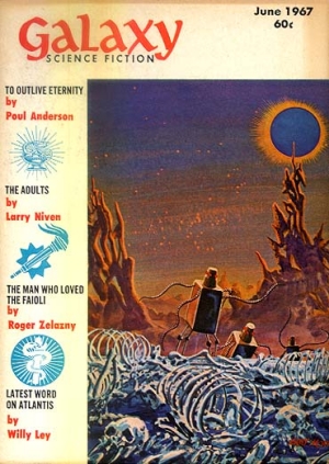
Image: What would become Tau Zero first appeared in shortened form as “To Outlive Eternity” in the pages of Galaxy in June, 1967.
The Bussard Ramjet Leonora Christine sets out for Beta Virginis, approximately 36 light years away. A mid-trip mishap robs the ship of its ability to slow down. Repairs are impossible unless they shut down the ramjet, but if the crew did that, they would instantly be exposed to lethal radiation. There’s no choice but to keep accelerating and hope that the ship will eventually encounter a region in the intergalactic depths with a sufficiently hard vacuum so that the ramjet could be safely shut down. They do find such a region and repair the ship.
Anderson then introduces the mother of all twists. The Leonora Christine has accelerated for so long that the crew discover relative to the universe a cosmological amount of time has elapsed. The universe is not ‘open’ but fits the re-collapse model, it is going for the big crunch. I know of no other science fiction novel with more extreme problem solving that this hard SF story.
Anderson’s cosmology for Tau Zero seems to come totally from George Gamow [28]. Gamow and his students did pioneering work on early time cosmology, an elaboration of earlier work done by Georges Lemaître. When Poul Anderson wrote the novel, he may have been aware that Big Bang cosmology had evolved beyond Gamow’s models …. However, having his starship eventually orbit the ‘Cosmic Egg’ or Ylem was a solution to the crew’s problem. Alas, even in Gamow’s cosmology the ‘Ylem’ is the universe, so no way to ‘orbit’ it. Poetic license for the sake of a Ripping Yarn! (An intersecting exercise is to see what the trajectory of the Leonora Christine‘s plot problem is in current accelerating universe cosmology.)
After Niven and Anderson, the Bussard Ramjet became common currency in science fiction, although it has faded somewhat in recent times. Recently a fusion ramjet, SunSeeker, appears as an integral part of the Bowl of Heaven series by Greg Benford and Larry Niven [29].
Final Thoughts
There seems to be a thread of pessimism about the Bussard Ramjet centered around drag on the ramjet due to interaction with the scoop field. This is an issue that Fishback deals with in his analysis; he shows one cannot just use a dipole magnetic field. A more complex collector field is needed. Fishback and Martin do show there is a fundamental physics limitation. Even using the strongest material theoretically possible, there is an upper limit to a mission Lorentz factor, probably equal to 10,000. Above this one will bust the scoop coil due to magnetic stress. The cosmological peril of the Leonora Christine depicted in Tau Zero is not physically possible.
The main show stopper for the ramjet is the engineering. There is no way with foreseeable technology to build all the components of an interstellar ram scoop starship. Several aspects should be revisited. (1) The source of the magnetic scoop field, Fishback [7] derived one, Cassenti elaborated another [20]; (2) the fusion reactor — the aneutronic fusion concept is direct conversion of fusion to energy [30]; (3) hybrid systems, especially laser-boosted ramjets.
Since basic physics does not rule a ramjet out, it is possible that an advanced civilization might build one. Freeman Dyson [31] pointed out many times that what we could not do might be done by some advanced civilization as long as the fundamental physics allows it. An interesting consequence of this is that interstellar ramjets may have been built and might have observable properties. Doppler-boosted waste heat from such ships might be observable. Plowing into HII regions in the galaxy, a starship’s magnetic scoop field might produce a bow-shock which could be observable. Isolated objects in this galaxy with Lorentz factors in the thousands would be unusual and if they are accelerating even more unusual.
The idea of picking up your fuel along the way in your journey across interstellar space may be the optimal solution to the mass ratio problem in interstellar flight. The interstellar ramjet warrants more technical study.
Appendix
Because Robert Bussard sketched a ramjet with a physical ‘funnel’ …all the many illustrations I have seen since seem to have some kind of ‘cow catcher’ on the front. Though it is reasonable that such a structure is the source of an electromagnetic device, I think it more likely that the ‘scoop’ field will be produced by a magnetic configuration that directs the incoming stream into the mouth of the reactor without any extra funnel-like forward structure. Here is a rough schematic done for me by artist Doug Potter. There is a ‘bulb’ representing the magnetic source field (maybe the parabolic magnetic field calculated by Fishback), a reactor section and an exhaust. Not a very elegant representation of the ramjet but a suggested configuration.
References
1. Bussard, R. W., and R. D. DeLauer. Nuclear Rocket Propulsion, McGraw-Hill, New York, 1958
2. L. R. Shepherd, “Interstellar Flight,” Journal of the British Interplanetary Society, 11, 4, July 1952
3. R.W. Bussard, “Galactic matter and interstellar flight,” Astronautica Acta 6 (1960) 179-195
4. C. Sagan, “Direct contact among galactic civilizations by relativistic interstellar spaceflight,” Planet. Space Sci. 11 (1963) 485-498
5. Sagan, Carl; Shklovskii, I. S. (1966). Intelligent Life in the Universe. Random House
6. Sänger, E., “Zur Flugmechanik der Photonenraketen.” Astronautica Acta 3 (1957), S. 89-99
7. Fishback J F, “Relativistic interstellar spaceflight,” Astronautica Acta 15 25-35, 1969
8. Anthony R. Martin; “Structural limitations on interstellar spaceflight,” Astronautica Acta, 16, 353-357 , 1971
9. Anthony R. Martin; “Magnetic intake limitations on interstellar ramjets,” Astronautica Acta 18, 1-10 , 1973
10. Whitmire, Daniel P., “Relativistic Spaceflight and the Catalytic Nuclear Ramjet” Acta Astronautica 2 (5-6): 497-509, 1975
11. Bond, Alan, “An Analysis of the Potential Performance of the Ram Augmented Interstellar Rocket,” Journal of the British Interplanetary Society, Vol. 27, p.674,1974
12. Powell, Conley, “Flight Dynamics of the Ram-Augmented Interstellar Rocket,” Journal of the British Interplanetary Society, Vol. 28, p.553, 1975
13. Jackson, A. A., “Some Considerations on the Antimatter and Fusion Ram Augmented Interstellar Rocket,” Journal of the British Interplanetary Society, v33, 117, 1980.
14. R.L. Forward, “Antimatter Propulsion”, Journal of the British Interplanetary Society, 35, pp. 391-395, 1982
15. Kammash, T., and Galbraith, D. L., “Antimatter-Driven-Fusion Propulsion for Solar System Exploration,” Journal of Propulsion and Power, Vol. 8, No. 3, 1992, pp. 644 – 649
16. Heppenheimer, T.A. (1978). “On the Infeasibility of Interstellar Ramjets”. Journal of the British Interplanetary Society 31: 222
17. Matloff, G.L., and A.J. Fennelly, “A Superconducting Ion Scoop and Its Application to Interstellar Flight”, Journal of the British Interplanetary Society, Vol. 27, pp. 663-673, 1974
18. Matloff, G.L., and A.J. Fennelly, “Interstellar Applications and Limitations of Several Electrostatic/Electromagnetic Ion Collection Techniques”, Journal of the British Interplanetary Society, Vol. 30, pp. 213-222, 1980
19. Matloff, G.L., and A.J. Fennelly , B. N , “Design Considerations for the Interstellar Ramjet,” 44th AIAA/ASME/SAE/ASEE Joint Propulsion Conference & Exhibit, 2008
20. Cassenti, B. N , “The Interstellar Ramjet,” 40th AIAA/ASME/SAE/ASEE Joint Propulsion Conference and Exhibit, 2004
21. Claude Semay and Bernard Silvestre-Brac, “The equation of motion of an interstellar Bussard ramjet,” European Journal of Physics 26(1):75, 2004
22. Claude Semay and Bernard Silvestre-Brac, “Equation of motion of an interstellar Bussard ramjet with radiation loss,” Acta Astronautica 61(10):817-822, 2007
23. Whitmire, D. and Jackson, A, “Laser Powered Interstellar Ramjet,” Journal of the British Interplanetary Society Vol. 30pp. 223-226, 1977
24. Mallove, E. F., and G.L. Matloff, The Starflight Handbook, Wiley, New York, 1989
25. Matloff, G., Deep-Space Probes, Praxis Publishing, Chichester, UK, 2000
26. Ian A Crawford, “Direct Exoplanet Investigation Using Interstellar Space Probes.” In Handbook of Exoplanets Springer 2017
27. Anderson, Poul. Tau Zero. New York: Lancer Books (1970)
28. George Gamow, The Creation of the Universe (1952)
29. Benford, G. and Niven, L., Bowl of Heaven series, Macmillan.
30. Benford, G., Private communication.
31. Dyson, F. J., “The search for extraterrestrial technology,” in Marshak, R.E. (ed), Perspectives in Modern Physics, Interscience Publishers, New York, pp. 641-655
WFIRST: Exoplanets in the Direction of Galactic Center
The Kepler mission gave us, along with plenty of exoplanetary scenarios, a statistical look at a particular patch of sky, one containing parts of Lyra, Cygnus and Draco. Some of the stars within that field were close (Gliese 1245 is just 15 light years out), but the intention was never to home in on nearby systems. Most of the Kepler stars ranged from 600 to 3,000 light years away. Instead, Kepler would produce an overview of planets around different stellar types, including some in the habitable zone of their stars.
As with all such observations, we’re limited by the methods chosen, which in Kepler’s case involved transits of the host star. TESS, the Transiting Exoplanet Survey Satellite, likewise uses the transit method, though with particular reference to broad sky coverage and close, bright stars. We can deploy the widely anticipated James Webb Space Telescope, to be launched next year, to follow up interesting finds, but let’s also consider how useful the Wide Field Infrared Survey Telescope (WFIRST) is going to be, for this instrument brings a new population of planets into the mix.
Not that WFIRST won’t be able to spot transits as well, but the real interest here is microlensing, a phenomenon a good deal less common than transits, but one holding the promise of finding planets far more distant than Kepler. Looking toward the passage of a star and planetary system in front of a background star, astronomers can catch the lensing effect produced by the warping of spacetime. That quick brightening can contain within it the signature of one or more planets.
As you would imagine, finding these occultations is tricky, for they don’t occur very often. David Bennett is head of the gravitational microlensing group at NASA’s Goddard Space Flight Center. Kepler monitored more than 150,000 stars in its primary mission, but WFIRST will have a lot more to play with, says Bennett :
“Microlensing signals from small planets are rare and brief, but they’re stronger than the signals from other methods. Since it’s a one-in-a-million event, the key to WFIRST finding low-mass planets is to search hundreds of millions of stars.”
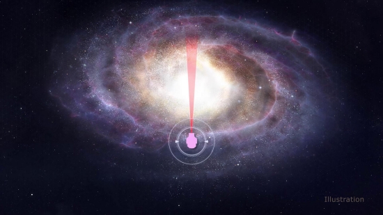
Image: WFIRST will make its microlensing observations in the direction of the center of the Milky Way galaxy. The higher density of stars will yield more exoplanet detections. Credit: NASA’s Goddard Space Flight Center/CI Lab.
Slated for launch in the mid-2020s, WFIRST will round out what we’ve learned from previous missions and different exoplanet detection methods. Radial velocity is sensitive to planets close to the host star and, with ever greater spectroscopic precision, can tease out information about smaller worlds further out. Transits are excellent for finding small worlds in tight orbits. What microlensing brings to the table are planets of all sizes — and perhaps even large moons — orbiting at a wide range of distances from the host, as far out as Uranus and Neptune and potentially much farther.
Here the bias, if we want to call it that, is toward planets from the habitable zone outward, fully complementing our other methods, which function so much better in inner systems. We have no idea how common ice giants are, but WFIRST should help us build the census. We go from Kepler’s 115 square degree field of view of stars typically within 1,000 light years to a 3 square degree field that, because it’s toward galactic center, will track 200 million stars. Their average distance will be in the range of 10,000 light years, far beyond the reach of other methods.
Microlensing has produced its share of planets — 86 so far — but bear in mind that the observations that have turned them up have been in visible light, which means that looking toward the center of the galaxy, shrouded in dust, has not been feasible. That’s beginning to change with the United Kingdom Infrared Telescope (UKIRT), which from its vantage in Hawaii has begun mapping the region. Data from UKIRT will help determine the WFIRST microlensing observation strategy.
Savannah Jacklin (Vanderbilt University) has led studies using UKIRT data:
“Our current survey with UKIRT is laying the groundwork so that WFIRST can implement the first space-based dedicated microlensing survey. Previous exoplanet missions expanded our knowledge of planetary systems, and WFIRST will move us a giant step closer to truly understanding how planets – particularly those within the habitable zones of their host stars – form and evolve.”
But WFIRST microlensing goes beyond exoplanet discovery to take in everything from black holes to neutron stars, brown dwarfs and ‘rogue’ planets that have been ejected from their planetary systems. TESS is currently tracking 200,000 stars over the entire sky. The infrared studies of WFIRST will dramatically add to what Kepler and TESS have given us, using machine learning tools now being refined by UKIRT to comb through the data. An overview of planetary populations at all distances from the host star, and with a target field containing hundreds of millions of stars, is the much desired result.
Getting Real with the Habitable Zone
Perhaps the most significant paper I have yet to read on the subject of habitable zones has emerged from the University of Oxford, with collateral help from the Lamb and Flag on nearby St. Giles St. (a stout place), along with two scientists who claim no affiliation other than ‘Earth.’ The paper defines the Really Habitable Zone, that region around a star within which acceptable gins and tonic are likely to be found. “We suggest that planets in the Really Habitable Zone be early targets for the JWST, because by the time that thing finally launches we’re all going to need a drink.” Which is so patently true that I can only nod with approval.
Adding that most habitable zone models now in play are defined by the need to justify the budget of the JWST to the US Congress, the authors proceed to note the difficulties in creating a habitable zone definition with which all astronomers can agree. What all astronomers can support, they argue, is a definition of what makes life worth living. Throw in a good infrastructure to support the distribution of limes and you are on your way.

The Really Habitable Zone (RHZ) defined here has a substantial history in the literature, as the authors note:
Astronomers have long been interested in alcohol. Shortly after the introduction of gin to the UK, Flamsteed made the first observations of Uranus but mistook it for a star; we suggest a connection between these two events. In the twentieth century, papers by Coburn (1932) and Phenix & Littell (1933) discuss the use of alcohols to treat photographic plates, though they remain silent on its use in treating astronomers. Ball et al. (1972) detected methanol, though this is – in space, as on Earth – clearly undrinkable. Luckily, Zuckerman et al. (1975) soon found ethanol.
The chain of reasoning is tight. The paper continues:
It is therefore clear that conditions which support the creation of decent beverages will also support astronomers, which is a working definition of civilization. The choice of gin and tonic is based on the work of Adams (Adams 1979), who hypothesised that a drink named something similar existed in 85% of civilizations.
Image: Much of the research for this paper was conducted at the Lamb and Flag in Oxford.
A Minimum Acceptable Gin and tonIC (MAGIC) is defined; here the authors do extol the value of citrus, but being British, they seem unwilling to acknowledge lime as the acidic vehicle of choice, allowing sliced lemon in ways that have bewildered many an American scientist at conferences in the UK. We can expect some spirited pushback from the States in response, as MAGIC is critical for the theoretical and observational definition of the Really Habitable Zone.
As to gin, juniper is acknowledged as the essential ingredient, and an exo-Juniper is defined, with the understanding that its tolerance for varied climatic conditions does not force strong limits on the RHZ, whereas what the authors call ‘ginspermia’ (the transport of juniper berries between the stars) is unlikely on planets with efficient harvesting and maximal gin production. The RHZ is, on the other hand, defined by the necessity for citrus fruits to thrive in a relatively narrow temperature range and a supply of H2O. The authors’ equation 1 encapsulates their assumptions on atmospheric modeling and planetary weather (the equation is, unfortuntely, too baroque to insert easily into the Centauri Dreams format).
The inner RHZ defined here is loosely based on ‘Recent Venus’ work available in the literature. Curiously, the outer edge coefficients of the RHZ equation appear to align with the founding years of a number of well-known gin distilleries, a fact the paper acknowledges but fails to follow up on. Thus the paper’s major shortcoming, described disarmingly by the authors themselves:
We had planned to carry out a statistical test to determine whether the populations of planets within and without the Really Habitable Zone were really different. However, the undergraduate student we’d expected to apply a Bayesian Machine Learning model has stopped answering our emails, so we merely suggest you follow astronomical tradition and look at the graph for a few seconds before drawing sweeping conclusions from it.
And here is the graph. Note that BHZ stands for Boring Habitable Zone, the authors’ term for more conventional models now in circulation:
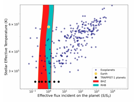
Image: This is Figure 1 from the paper. Caption: As this figure shows, the Earth (lemon) is worryingly close to the outermost edge of the Really Habitable Zone (teal blue region). One might think that this is cause for panic, however, the authors have extensively tested and verified the existence of gins and tonic on Earth. Our vigilance in this matter is (nearly) unceasing. Credit: Pedbost et al.
This compelling work includes an interesting section on observational prospects for detecting gins and tonic on exoplanets (“As with many exoplanet papers, this one includes a section on wildly infeasible future observations which, though difficult, would undoubtedly have enormous scientific impact”). The authors assume 1 bar atmospheric pressure in their calculations, for reasons that should be apparent, and evaluate methodologies for detection of both gin and citrus, assuming tonic is ubiquitous because gin without it is “literally unthinkable.” How true.
The paper is Pedbost et al. (with what I take to be a liberal contribution from the ever reliable Chris Lintott), “Defining the Really Habitable Zone,” available as a preprint. Thanks for the pointer goes to my friend Ashley Baldwin, who knows the value of the occasional jest in dire times.
Deep Time: Exoplanet Atmospheres in Perspective
As we improve our instrumentation, the search for worlds where life can flourish will generate more and more Earth-sized targets for extended investigation. Here time plays an interesting role, for our own planet seen two billion years ago would present a different aspect than the Earth of today. Atmospheres evolve, a fact that Lisa Kaltenegger has studied in a series of papers in recent years, working with colleagues at Cornell’s Carl Sagan Institute, where she is director. The result is a series of spectral templates applicable to Earth-like planets at various stages of evolution.
We have only one known example of a living planet to work with, so Kaltenegger’s atmospheric models are designed to match the Earth at different stages of development. The prebiotic Earth of 3.9 billion years ago is saturated with carbon dioxide, while what the paper refers to as Epoch 2, some 3.5 billion years ago, is a world without oxygen. Three more epochs can be defined covering the rise of atmospheric oxygen, from levels below 1 percent beginning about 2.4 billion years ago (the Grand Oxygenation Event) to 10 percent oxygen (the Neoproterozoic Oxygenation Event) and the modern Earth atmosphere with oxygen levels at 21 percent.

“Using our own Earth as the key, we modeled five distinct Earth epochs to provide a template for how we can characterize a potential exo-Earth – from a young, prebiotic Earth to our modern world,” Kaltenegger said. “The models also allow us to explore at what point in Earth’s evolution a distant observer could identify life on the universe’s ‘pale blue dots’ and other worlds like them.”
Image: Lisa Kaltenegger, director of the Carl Sagan Institute at Cornell and Associate Professor in Astronomy. Credit: Cornell University.
The resulting database draws on a solar evolution model that establishes the solar flux through the epochs described, all applied to a hypothesized planet with the same mass and radius as Earth orbiting at 1 AU from an evolving Sun. Note that in previous work, Kaltenegger and colleagues have developed reflection and emission spectra of Earth through its geological history, and have also applied these data to different classes of host stars. This model is different, in that it’s focused on transmission spectra, meaning we’re looking at what data a transiting planet would present to our spectrographs as the light of its host star passed through its atmosphere.
The high-resolution database that comes out of this work goes through visible wavelengths into the infrared (0.4-20 μm) through geological time. Transmission spectra of this kind are the current tool for probing exoplanet atmospheres and may well be the first derived from Earth-sized worlds in habitable zone orbits.
From the paper:
Throughout the atmospheric evolution of our Earth, different absorption features dominate Earth’s transmission spectrum…with CH4 and CO2 being dominant in early Earth models, where they are more abundant. O2 and O3 spectral features become stronger with increasing abundance during the rise of oxygen (Epoch 3-5). High-resolution (λ/Δλ = 100,000) spectral features that indicate life on Earth —the combination of O2 or O3 with a reducing gas like CH4 or N2O—can be detected for oxygen levels as low as 0.01 present atmospheric levels (0.21% O2), which correspond to a Neoproterozoic Earth model and a time about one to two billion years ago in Earth’s history.
The authors used a climate-photochemistry tool called EXO-Prime to compile the database, noting that its results have been validated for visible to infrared wavelengths when Earth is observed as an exoplanet. We’ve talked in the past about the EPOXI mission’s look back at Earth (see EPOXI: Clues to Terrestrial Worlds), but we also have data from Mars Global Surveyor and numerous Earthshine observations that have demonstrated the tool is robust. The results clearly show how different absorption features dominate the Earth’s spectrum through the course of atmospheric change.
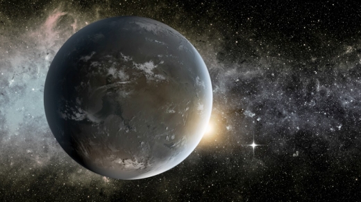
Image: This artistic depiction shows exoplanet Kepler-62f, a rocky super-Earth size planet, located about 1,200 light-years from Earth in the constellation Lyra. Kepler-62f may be what a prebiotic Earth may have looked like. Other exoplanets may look similar. Credit: NASA Ames/JPL-Caltech.
For those wanting to explore these issues further, the high-resolution transmission spectra database can be found online at www.carlsaganinstitute.org/data. The authors see it as a tool for data interpretation as well as optimizing observation strategy and training data retrieval methods as new instruments become available. The work is applicable not only to the introduction of the ground-based Extremely Large Telescopes like the Giant Magellan Telescope and the Thirty Meter Telescope, but also space-based missions like the James Webb Space Telescope as well as future mission concepts like LUVOIR (Large UV Optical Infrared telescope) and HabEx (Habitable Exoplanet Observatory).
Kaltenegger notes that these telescopes will be identifying Earth-like planets out to about 100 light years:
“Once the exoplanet transits and blocks out part of its host star, we can decipher its atmospheric spectral signatures. Using Earth’s geologic history as a key, we can more easily spot the chemical signs of life on the distant exoplanets…Our transmission spectra show atmospheric features, which would show a remote observer that Earth had a biosphere as early as about 2 billion years ago.”
The paper is Kaltenegger et al., “High-resolution Transmission Spectra of Earth Through Geological Time,” Astrophysical Journal Letters Vol. 892, No. 1 (26 March 2020). Abstract.
Introducing the Q-Drive: A concept that offers the possibility of interstellar flight
If Breakthrough Starshot is tackling the question of velocities at a substantial percentage of lightspeed, what do we do about the payload question? A chip-sized spacecraft is challenging in terms of instrumentation and communications, not to mention power. Enter Jeff Greason’s Q-Drive, with an entirely different take on high velocity missions within the Solar System and beyond it. Drawing its energies from the medium to deploy an inert propellant, the Q-Drive ups the payload enormously. But can it be engineered? Alex Tolley has been doing a deep dive on the concept and talking to Dr. Greason about the possibilities, out of which today’s essay has emerged. A Centauri Dreams regular, Alex has a history of innovative propulsion work, and with Brian McConnell is co-author of A Design for a Reusable Water-Based Spacecraft Known as the Spacecoach (Springer, 2016),
by Alex Tolley
Technical University of Munich for Project Icarus. Credit: Adrian Mann.
The interstellar probe coasted at 4% c after her fusion drive first stage was spent. It massed 50,000 kg, mostly propellant water ice stored as a conical shield ahead of the probe that did double duty as a particle shield. The probe extended a spine, several hundred kilometers in length behind the shield. Then the plasma magnet sails at each end started to cycle, using just the power from a small nuclear generator. The magsails captured and extracted power from the ISM streaming by. This powered the ionization and ejection of the propellant. Ejected at the streaming velocity of the ISM, the probe steadily increased in velocity, eventually reaching 20% c after exhausting 48,000 kg of propellant. The probe, targeted at Proxima Centauri, would reach its destination in less than 20 years. It wouldn’t be the first to reach that system, the Breakthrough microsails had done that decades earlier, but this probe was the first with the scientific payload to make a real survey of the system and collect data from its habitable world.
(sound of a needle skidding across a vinyl record). Wait, what? How can a ship accelerate to 20% c without expending massive amounts of power from an onboard power plant, or an intense external power beam from the solar system?
In a previous article, I explained the plasma magnet drive, a magsail technology that did not require a large physical sail structure, but rather a compact electromechanical engine whose magnetic sail size was dependent on the power and the surrounding medium’s plasma density.
Like other magsail and electric sail designs, the plasma magnet could only run before the solar wind, making only outward bound trips and a velocity limited by the wind speed. This inherently limited the missions that a magsail could perform compared to a photon sail. Where it excelled was the thrust was not dependent on the distance from the sun that severely limits solar sail thrust, and therefore this made the plasma magnet sail particularly suited to missions to the outer planets and beyond.
Jeff Greason has since considered how the plasma magnet could be decelerated to allow the spacecraft to orbit a target in the outer system. Following the classic formulations of Fritz Zwicky, Greason considered whether the spacecraft could use onboard mass but external energy to achieve this goal. This external energy was to be extracted from the external medium, not solar or beamed energy, allowing it to operate anywhere where there was a medium moving relative to the vehicle.
The approach to achieve this was to use the momentum and energy of a plasma stream flowing past the ship and using that energy to transfer momentum to an onboard propellant to drive the ship. That plasma stream would be the solar wind inside the solar system (or another star system), and an ionized interstellar medium once beyond the heliosphere.
Counterintuitively, such a propulsion system can work in principle. By ejecting the reaction mass, the ship’s kinetic energy energy is maintained by a smaller mass, and therefore increases its velocity. There is no change in the ship’s kinetic energy, just an adjustment of the ship’s mass and velocity to keep the energy constant.
Box 1 shows that net momentum (and force) can be attained when the energy of the drag medium and propellant thrust are equal. However this simple momentum exchange would not be feasible as a drive as the ejection mass would have to be greater than the intercepted medium resulting in very high mass ratios. In contrast, the Q-Drive, achieves a net thrust with a propellant mass flow far less than the medium passing by the craft, resulting in a low mass ratio yet high performance in terms of velocity increase.
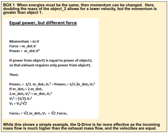
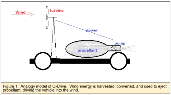
Figure 1 shows the principle of the Q-Drive using a simple terrestrial vehicle analogy. Wind blowing through a turbine generates energy that is then used to eject onboard propellant. If the energy extracted from the wind is used to eject the propellant, in principle the onboard propellant mass flow can be lower than the mass of air passing through the turbine. The propellant’s exhaust velocity is matched to that of the wind, and under these conditions, the thrust can be greater than the drag, allowing the vehicle to move forward into the wind.
Box 2 below shows the basic equations for the Q-Drive.
Let me draw your attention to equations 1 & 2, the drag and thrust forces. The drag force is dependent on the velocity of the wind or the ship moving through the wind which affects the mass flow of the medium. However, it is the change in velocity of the medium as it passes through the energy harvesting mechanism rather than the wind velocity itself that completes this equation. Compare that to the thrust from the propellant where the mass flow is dependent on the square of the exhaust velocity. When the velocity of the ship and the exhaust are equal, the ratio of the mass flows is dependent on the ratio of the change in velocity (delta V) of the medium and the exhaust velocity. The lower the delta V of the medium as the energy is extracted from it, the lower the mass flow of the propellant. As long as the delta V of the medium is greater than zero, as the delta V approaches zero, the mass of the stream of medium is greater than the mass flow of the propellant. Conversely, as the delta V approaches the velocity of the medium, i.e. slowing it to a dead stop relative to the ship, the closer the medium and exhaust mass flows become.
Equations 3 and 7 are for the power delivered by the medium and the propellant thrust. As the power needed for generating the thrust cannot be higher than than delivered by the medium, at 100% conversion the power of each must be equal. As can be seen, the power generated by the energy harvesting is the drag force multiplied by the speed of the medium. However, the power to generate the thrust is ½ the force of the thrust multiplied by the exhaust velocity, which is the same as the velocity of the medium. Therefore the thrust is twice that of the drag force and therefore a net thrust equal to the drag force is achieved [equation 9]. [Because the sail area must be very large to capture the thin solar wind and the even more rarified ISM, the drag force on the ship itself can be discounted.]
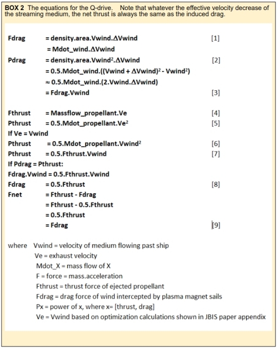
Because the power delivered from the external medium increases as the ship increases in velocity, so does the delivered power, which in turn is used to increase the exhaust velocity to match. This is very different from our normal expectations of powering vehicles. Because of this, the Q-Drive can continue to accelerate a ship for as long as it can continue to exhaust propellant.
Figure 2 shows the final velocity versus the ship’s mass ratio performance of the Q-Drive compared to a rocket with a fixed exhaust velocity, and the rocket equation using a variable exhaust but with the thrust reduced by 50% to match the Q-drive net thrust equaling 50% of the propellant thrust. With a mass ratio below 10, a rocket with an exhaust equal to the absolute wind velocity would marginally outperform the Q-drive, although it would need its own power source to run, such as a solar array or nuclear reactor. Beyond that, the Q-drive rapidly outperforms the rocket. This is primarily because as the vehicle accelerates, the increased power harvested from the wind is used to commensurately increase the exhaust velocity. If a rocket could do this, for example like the VASIMR drive, the performance curve is the same. However, the Q-drive does not need a huge power supply to work, and therefore offers a potential for very high velocity without needing a matching power supply.
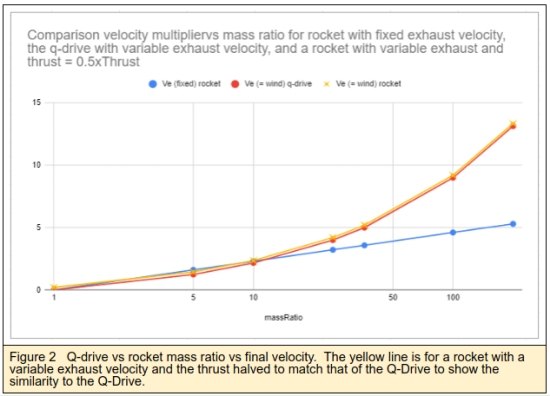
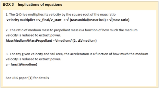
Equation A16 [1] and Box 3 equation 1 show that the Q-Drive has a velocity multiplier that is the square root of the mass ratio. This is highly favorable compared to the rocket equation. The equations 2 and 3 in Box 3 show that the required propellant and hence mass ratio is reduced the less the medium velocity is reduced to extract power. However, reducing the delta V of the medium also reduced the acceleration of the craft. This implies that the design of the ship will be dependent on mission requirements rather than some fixed optimization.
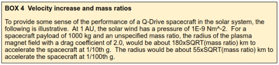
Box 4 provides some illustrative values for the size of the mag sails in the solar system for the Q-Drive and the expected performance for a 1 tonne craft. While the magnetic sail radii are large, they are achievable and allow for relatively high acceleration. As explained in [4], the plasma magnet sails increase in size as the medium density decreases, maintaining the forces on the sail. Once in interstellar space, the ISM is yet more rarefied and the sails have to commensurately expand.
How might the plasma medium’s energy be harvested?
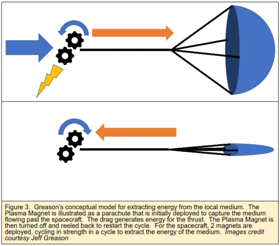
The wind turbine shown in figure 1 is replaced by an arrangement of the plasma magnet sails. To harvest the energy of the medium, it is useful to conceptualize the plasma magnet sail as a parachute that slows the wind to run a generator. At the end of this power stroke, the parachute is collapsed and rewound to the starting point to start the next power cycle. This is illustrated in figure 3. A ship would have 2 plasma magnet sails that cycle their magnetic fields at each end of a long spine that is aligned with the wind direction to mimic this mechanism. The harvested energy is then used to eject propellant so that the propellant exhaust velocity is optimally the same as the medium wind speed. By balancing the captured power with that needed to eject propellant, the ship needs no dedicated onboard power beyond that for maintenance of other systems, for example, powering the magnetic sails.
Within the solar system, the Q-Drive could therefore push a ship towards the sun into the solar wind, as well as away from the sun with the solar wind at its back. Ejecting propellant ahead of the ship on an outward bound journey would allow the ship to decelerate. Ejecting the propellant ahead of the ship as it faced the solar wind would allow the ship to fall towards the sun. In both cases, the maximum velocity is about the 400 km/s of the peak density velocity of the solar wind.
Can the drive achieve velocities greater than the solar wind?
With pure drag sails, whether photon or magnetic, the maximum velocity is the same as the medium pushing on the sail. For a magnetic sail, this is the bulk velocity of the solar wind, about 400 km/s at the sun’s equator, and 700 km/s at the sun’s poles.
Unlike drag sails, the Q-Drive can achieve velocities greater than the medium, e.g. the solar wind. As long as the wind is flowing into the bow of the ship, the ship can accelerate indefinitely until the propellant is exhausted. The limitation is that this can only happen while the ship is facing into the wind (or the wind vector has a forward facing component). In the solar system, this requires that there is sufficient distance to allow the ship to accelerate until its velocity is higher than the solar wind before it flies past the sun. Once past perihelion, the ship is now running into the solar wind from behind, and can therefore keep accelerating.
What performance might be achievable?
To indicate the possible performance of the Q-drive in the solar system, 2 missions are explored, both requiring powered flight into the solar wind.
Two Solar System Missions
1. Mercury Rendezvous
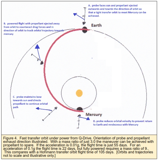
To reach Mercury quickly requires the probe to reduce its orbital speed around the sun to drop down to Mercury’s orbit and then reduce velocity further to allow orbital insertion. The Q-Drive ship points its bow towards the sun, and ejects propellant off-axis. This quickly pushed the probe into a fast trajectory towards the sun. Further propellant ejection is required to prevent the probe from a fast return trajectory and to remain in Mercury’s sun orbital path. From there a mix of propellant ejection and simple drag alone can be used to place the probe in orbit around Mercury. Flight time is of the order of 55 days. Figure 4 illustrates the maneuver.
2. Sundiver with Triton Flyby
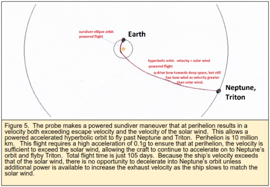
The recent Centauri Dreams post on a proposed flyby mission to Triton indicated a flight time of 12 years using gravity assists from Earth, Venus, and Jupiter.. The Q-Drive could reduce most of that flight time using a sundiver approach. Figure 5 shows the possible flight path. The Q-Drive powers towards the sun against the solar wind. It must have a high enough acceleration to ensure that at perihelion it is now traveling faster than the solar wind. This allows it to now continue on a hyperbolic trajectory continually accelerating until its propellant is exhausted.
This sundiver maneuver allows the Q-Drive craft to fly downwind faster than the wind.
For a ship outward bound beyond the heliosphere, the ISM medium is experienced as a wind coming from the bow, While extremely tenuous, there is enough medium to extract the energy for continued acceleration as long as the ship has ejectable mass.
Up to this point, I have been careful to state this works IN PRINCIPLE. In practice there are some very severe engineering challenges. The first is to be able to extract energy from the drag of the plasma winds with sufficient efficiency to generate the needed power for propellant ejection. The second is to be able to eject propellant with a velocity that matches the speed of the vehicle, IOW, the exhaust velocity must match the vehicle’s velocity, unlike the constant exhaust velocity of a rocket. If the engines to eject propellant can only eject mass at a constant velocity, the delta V of the drive would look more like a conventional rocket, with a natural logarithm function of the mass flow. The ship would still be able to extract energy from the medium, but the mass ratio would have to be very much higher. The chart in Figure 2 shows the difference between a fixed velocity exhaust and the Q-Drive with variable velocity.
The engineering issues to turn the Q-Drive into hardware are formidable. To extract the energy of the plasma medium whether solar wind or ISM, with high efficiency, is non-trivial. Greason’s idea is to have 2 plasma magnet drag sails at each end of the probe’s spine that cycle in power to extract the energy. The model is rather like a parachute that is open to create drag to push on the parachute to run a generator, then collapse the parachute to release the trapped medium and restart it at the bow (see figure 3). Whether this is sufficient to create the needed energy extraction efficiency will need to be worked out. If the efficiencies are like those of a vertical axis wind turbine that works like drag engines, the efficiencies will be far too low. The efficiency would need to be higher than that of horizontal axis wind turbines to reduce the mass penalties for the propellant. It can be readily seen that if the efficiencies combine to be lower than 50%, then the Q-Drive effectively drops back into the regime illustrated in Box 1, that is that the mass of propellant must become larger than the medium and ejected more slowly. This hugely raises the mass ratio of the craft and in turn reduces its performance.
The second issue is how to eject the propellant to match the velocity of the medium streaming over the probe. Current electric engines have exhaust velocities in the 10s of km/s. Theoretical electric engines might manage the solar wind velocity. Efficiencies of ion drives are in the 50% range at present. To reach a fraction of light speed for the interstellar mission is orders of difficulty harder. Greason suggests something like a magnetic field particle accelerator that operates the length of the ship’s spine. Existing particle accelerators have low efficiencies, so this may present another very significant engineering challenge. If the exhaust velocity cannot be matched to the speed of the ship through the medium, the performance looks much more like a rocket, with velocity increases that depend on the natural logarithm of the mass ratio, rather than the square root. For the interstellar mission, increasing the velocity from 4% to 20% light speed would require a mass ratio of not just 25, but rather closer to 150.
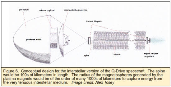
Figure 6 shows my attempt to illustrate a conceptual Q-Drive powered spacecraft for interstellar flight. The propellant is at the front to act as a particle shield in the ISM. There is a science platform and communication module behind this propellant shield. Behind stretches a many kilometers long spine that has a plasma magnet at either end to harvest the energy in the ISM and to accelerate the propellant. Waste heat is handled by the radiator along this spine.
In summary, the Q-Drive offers an interesting path to high velocity missions both intra-system and interstellar, with much larger payloads than the Breakthrough Starshot missions, but with anticipated engineering challenges comparable with other exotic drives such as antimatter engines. The elegance of the Q-Drive is the capability of drawing the propulsion energy from the medium, so that the propellant can be common inert material such as water or hydrogen.
The conversion of the medium’s momentum to net thrust is more efficient than a rocket with constant exhaust velocity using onboard power allowing far higher velocities with equivalent mass ratios. The two example missions show the substantial improvements in mission time for both and inner system rendezvous and an outer system flyby. The Q-Drive also offers the intriguing possibility of interstellar missions with reasonable scientific and communication payloads that are not heroic feats of miniaturization.
References
1. Greason J. “A Reaction Drive Powered by External Dynamic Pressure” (2019) JBIS v72 pp146-152.
2. Greason J. ibid. equation A4 p151.
3. Greason J. “A Reaction Drive Powered by External Dynamic Pressure” (2019) TVIW video https://youtu.be/86z42y7DEAk
4. Tolley A. “The Plasma Magnet Drive: A Simple, Cheap Drive for the Solar System and Beyond” (2017) https://www.centauri-dreams.org/2017/12/29/the-plasma-magnet-drive-a-simple-cheap-drive-for-the-solar-system-and-beyond/
5. Zwicky F. The Fundamentals of Power (1946). Manuscript for the International Congress of Applied Mechanics in Paris, September 22-29, 1946.
Follow with RSS or E-Mail
