Centauri Dreams
Imagining and Planning Interstellar Exploration
Can Life Survive a Star’s Red Giant Phase?
If we ever find life on a planet orbiting a white dwarf star, it will be life that has emerged only after the red giant phase has passed and the white dwarf has emerged as a stellar relic. That’s the conclusion of a study being discussed today at the National Astronomy Meeting of Britain’s Royal Astronomical Society, which convened online due to COVID concerns. The work is also recently published in Monthly Notices of the Royal Astronomical Society.
At issue is the damage caused by powerful stellar winds that occur as a star makes the transition from red giant to white dwarf stage. This is the scenario that awaits our own Sun, which should swell to red giant status in roughly five billion years, eventually becoming a dense white dwarf about the size of the Earth. We’ve speculated in these pages about life surviving this phase of stellar evolution, but the study, in the hands of Dimitri Veras (Warwick University) concludes that this is all but impossible.
We know that the Earth is protected by a magnetosphere that thwarts atmospheric depletion by channeling harmful particles along magnetic field lines. You would think that a magnetosphere would ease this kind of erosion in the far future for those planets that have one (Mars, for example, does not) but the stellar winds of the evolving star will be far stronger than the Sun’s today. The authors modeled the winds from eleven different kinds of stars in a range of masses. They find this:
The plot shows that an exo-Jovian analogue would just reach the threshold for hosting a magnetopause at some point during giant branch evolution. However, much higher fields would be required to maintain any magnetopause throughout these giant branch phases. For terrestrial and potentially habitable planets, any protection previously afforded by the magnetosphere would effectively disappear. This lack of protection, compounded with orbital expansion and varying stellar luminosities, suggest that life would be challenged to survive throughout the giant branch phases of stellar evolution.
Could scenarios emerge in which moons around the gas giants maintain life under an ice crust? It’s hard to see how. Veras, working with Aline Vidotto (Trinity College, Dublin) points out that a habitable zone supporting liquid water would move from some 150 million kilometers from the Sun to up to 6 billion kilometers, pushing it beyond the orbit of Neptune. Planets can migrate during this phase, but the paper argues that the habitable zone moves outward faster than the planet, a likely fatal threat. Thus life around a white dwarf will need to start over.
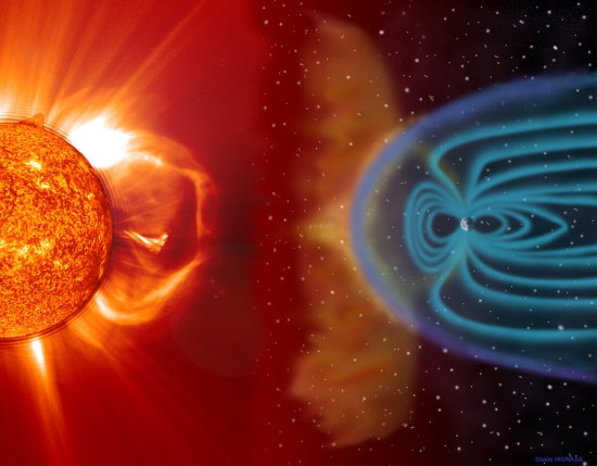
Image: An illustration of material being ejected from the Sun (left) interacting with the magnetosphere of the Earth (right). When the Sun evolves to become a red giant star, the Earth may be swallowed by our star’s atmosphere, and with a much more unstable solar wind, even the resilient and protective magnetospheres of the giant outer planets may be stripped away. MSFC / NASA. Licence type Attribution (CC BY 4.0).
Thus the movement of the habitable zone outward and the difficulty in maintaining a magnetosphere throughout this phase of stellar evolution make preserving habitability extremely unlikely. The authors’ model shows that the strong stellar wind combines with the expanding orbits of surviving planets to first shrink and then expand the magnetosphere of a planet over time. It would take a magnetic field 100 times stronger than Jupiter’s to maintain a stable magnetosphere all the way through the transition of red giant to white dwarf:
“We find that a planetary magnetosphere will always be quashed at some point during the giant branch phases, unless the planet’s magnetic field strength is at least two orders of magnitude higher than Jupiter’s current value.”
And afterwards? White dwarfs do not emit stellar winds, so that threat disappears. Any life we find around a white dwarf will doubtless have developed during the white dwarf phase. If such exists, we may be able to detect its biomarkers through future space missions — recall that white dwarfs are roughly the size of the Earth, and a transiting planet would produce profound transit depth and would seemingly be an ideal target for transmission spectroscopy, in which we analyze the components of a planetary atmosphere as starlight passes through it.
Most of the exoplanets we know about orbit main sequence stars, but about 100 are known to orbit red giants, and at least four have been found orbiting white dwarf stars. These worlds are survivors of stellar evolution and thus useful as benchmarks in tracing the lifetime of their systems. Two of the white dwarf planets, says Veras, are close to their star’s habitable zone, an indication of planet migration showing that an Earth-sized planet could exist in such an orbit. And he adds:
“These examples show that giant planets can approach very close to the habitable zone. The habitable zone for a white dwarf is very close to the star because they emit much less light than a Sun-like star. However, white dwarfs are also very steady stars as they have no winds. A planet that’s parked in the white dwarf habitable zone could remain there for billions of years, allowing time for life to develop provided that the conditions are suitable.”
The paper is Veras & Vidotto, “Planetary magnetosphere evolution around post-main-sequence stars,” Monthly Notices of the Royal Astronomical Society Vol. 506, Issue 2 (September 2021), pp. 1697-1703. Abstract / Preprint.

The Io Trigger: Radio Waves at Jupiter
Our recent discussion about Europa (Europa: Below the Impact Zone) has me thinking about those tempting Galilean moons and the problems they present for exploration. With a magnetic field 20,000 times stronger than Earth’s, Jupiter is a radiation generator. Worlds like Europa may well have a sanctuary for life beneath the ice, but exploring the surface will demand powerful radiation shielding for sensitive equipment, not to mention the problem of trying to protect a fragile human in that environment.
Radiation at Europa’s surface is about 5.4 Sv (540 rem), although to be sure it seems to vary, with the highest radiation areas being found near the equator, lessening toward the poles. In human terms, that’s 1800 times the average annual sea-level dose. Europa is clearly a place for robotic exploration rather than astronaut boots on the ground.
Jupiter offers up an environment where the solar wind, hurling electrically charged particles at ever-shifting velocities, interacts with the powerful magnetosphere, stretching it out almost 1000 kilometers away from the Sun. It’s essential that we learn more about the behavior of the magnetic fields generated by gas giants, and on that score new work out of Goddard Space Flight Center offers some insight. GSFC’s Yasmina Martos and team have been using the inner Galilean moon, Io, as a probe, studying what sets off one type of radio emissions known to emanate from Jupiter.
Io’s volcanoes have been observed since the first Voyager flyby, driven by internal heat as the moon experiences the gravitational pull not only of Jupiter but neighboring large moons. Gas and particles released by this activity are ionized and swiftly captured by Jupiter’s magnetic field, being accelerated along the field toward the Jovian poles.
Out of this we get decametric radio emissions (DAM) as electrons spiral in the magnetic field, waves that the Juno spacecraft’s Juno Waves Instrument has been detecting. Jupiter also produces radio waves at centimeter and decimeter wavelengths, caused by atmospheric phenomenon as well as activity in the magnetosphere apart from the Io interactions. The planet is, in fact, the noisiest radio emitter in the Solar System apart from the Sun. Homing in on the Io emissions, the GSFC work deploys a new magnetic field model with higher accuracy near the moon and targets the particular geometric configurations of planet and moon needed for Juno to detect the emissions.
Studying the radio emissions mediated by Io doesn’t help us cope with the radiation problem, but it does offer clues about this particular magnetosphere, a phenomenon we’ll come to know much better as future missions arrive. The researchers, reporting in the Journal of Geophysical Research: Planets, found that the decameter radio waves are controlled by not just the strength but the shape of Jupiter’s magnetic field. They emerge from a cone-like space thus formed, so that the spacecraft can only receive the radio signal when Jupiter’s rotation moves that cone across the instrument. The effect is similar to a lighthouse beacon sweeping out to sea.
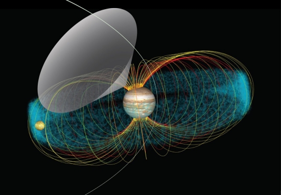
Image: The multicolored lines in this conceptual image represent the magnetic field lines that link Io’s orbit with Jupiter’s atmosphere. Radio waves emerge from the source and propagate along the walls of a hollow cone (gray area). Juno, its orbit represented by the white line crossing the cone, receives the signal when Jupiter’s rotation sweeps that cone over the spacecraft. Credit: NASA/GSFC/Jay Friedlander.
I can remember trying to pick up radio emissions from Jupiter with my first shortwave receiving set — they’ve been a known phenomenon since 1955, detectable from Earth at between 10 and 40 MHz. What we get thanks to the Juno observations is a clarification about why decametric radio waves originating in the northern hemisphere seem more abundant than those from the southern. The paper explains for the first time the particular geometric configurations producing these effects. The authors offer up a plain language summary to go along with the paper’s abstract, from which this:
Thanks to Juno, the geometry of the magnetic field has been better constrained as waves and magnetic field data have been continuously collected within the Jovian environment since July 2016. In this study, we estimate where the radio waves generate and the energy of the electrons that generate these waves, which is up to 23 times higher than previously proposed. We ultimately demonstrate that the geometry of Jupiter’s magnetic field is a primary controller for the higher observation likelihood of radio wave groups originating in the northern hemisphere relative to those originating in the southern hemisphere.
Video: The decametric radio emissions triggered by the interaction of Io with Jupiter’s magnetic field. The Waves instrument on Juno detects radio signals whenever Juno’s trajectory crosses into the beam which is a cone-shaped pattern. This beam pattern is similar to a flashlight that is only emitting a ring of light rather than a full beam. Juno scientists then translate the radio emission detected to a frequency within the audible range of the human ear. Credit: University of Iowa/SwRI/NASA.
What a fascinating place the Jovian system is. Learning the precise locations within the magnetosphere where the decametric emissions originate helps to pin down the needed magnetic field strength and electron density to fit the Juno data. “The radio emission is likely constant,” says Martos, “but Juno has to be in the right spot to listen.”
The paper is Martos et al, “Juno Reveals New Insights Into Io?Related Decameter Radio Emissions,” Journal of Geophysical Research: Planets (18 June 2020). Abstract.

Huge Comet Found to be Active
An interstellar freebie like ‘Oumuamua or 2I/Borisov is priceless. We don’t need to travel light years to see it because it comes to us. Although we’re expecting to find a lot more such objects as instruments like the Vera Rubin Observatory come online, right now only two are known to have passed through our system. But only slightly less inaccessible places like the Oort Cloud also bring gifts in the form of long-period comets, and I don’t want the advent of C/2014 UN271 Bernardinelli-Bernstein to go unnoticed in these pages, given its startling size and already detected activity.
Pedro Bernardinelli (University of Pennsylvania), who along with colleague Gary Bernstein discovered the comet, estimates its nucleus as being between 100 and 200 kilometers (62 and 125 miles) long. This dwarfs Hale-Bopp, and Colin Snodgrass (University of Edinburgh) is quoted in the New York Times as saying: “With a reasonable degree of certainty, it’s the biggest comet that we’ve ever seen.”
The discovery involved reprocessing data from the Dark Energy Survey, data that had been acquired via the 4-meter Blanco instrument at Cerro Tololo in Chile between 2013 and 2019. Bernardinelli and Bernstein announced the find in June of this year.
C/2014 UN271 was at roughly the distance of Neptune when first acquired in the data, although it is now about 20 AU out, or twice the distance of Saturn. While there was no statement about activity on the comet when the discovery was announced, astronomers at Las Cumbres Observatory quickly turned their network of telescopes on the object.
Las Cumbres offers a globally distributed network of telescopes with 24-hour robotic operation that is finely tuned to detect transients. Its instruments have now revealed that C/2014 UN271 is active, with the 1-meter LCO telescope at the South African Astronomical Observatory returning images that, in keeping with the international flavor of the observing effort, drew the attention of astronomers in New Zealand.
Thus Michele Bannister (New Zealand’s University of Canterbury):
“Since we’re a team based all around the world, it just happened that it was my afternoon, while the other folks were asleep. The first image had the comet obscured by a satellite streak and my heart sank. But then the others were clear enough and gosh: there it was, definitely a beautiful little fuzzy dot, not at all crisp like its neighbouring stars!”
Comet C/2014 UN271 was indeed active, that fuzzy dot indicating a coma. Volatile ices, likely carbon dioxide and carbon monoxide, were already reacting to the scant sunlight available. The coma was active even with the comet almost three billion kilometers from the Sun. No comet has ever been observed to be active this far from Sol.
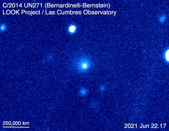
Image: Comet C/2014 UN271 (Bernardinelli-Bernstein), as seen in a synthetic color composite image made with the Las Cumbres Observatory 1-meter telescope at Sutherland, South Africa, on 22 June 2021. The diffuse cloud is the comet’s coma. Credit: LOOK/LCO.
This is one useful object, particularly since it was discovered early in its entry into the realm of the planets. It should offer astronomers over a decade of observing time. Perihelion is not expected until 2031, although when it comes, the comet will still be well beyond Saturn. Its orbit is now projected to take three million years to complete.
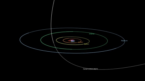
Image: An orbital diagram showing the path of Comet C/2014 UN271 (Bernardinelli-Bernstein) through the Solar System. The comets’ path is shown in gray when it is below the plane of the planets and in bold white when it is above the plane. Credit: NASA.
The discovery of activity on C/2014 UN271 draws attention to the LOOK Project now active at Las Cumbres. LOOK stands for LCO Outbursting Objects Key, an effort that investigates unexpected brightening of comets through burst activity and other aspects of comet evolution. Out of all this we should get a better understanding of comet outbursts, of which C/2014 UN271 is offering such a tantalizing sample.
These findings should also feed into future space missions like the European Space Agency’s Comet Interceptor, using data from this and other wide field surveys. Las Cumbres staff scientist Tim Lister explains:
“There are now a large number of surveys, such as the Zwicky Transient Facility and the upcoming Vera C. Rubin Observatory, that are monitoring parts of the sky every night. These surveys can provide alerts if one of the comets changes brightness suddenly and then we can trigger the robotic telescopes of LCO to get us more detailed data and a longer look at the changing comet while the survey moves onto other areas of the sky. The robotic telescopes and sophisticated software of LCO allow us to get images of a new event within 15 minutes of an alert. This lets us really study these outbursts as they evolve.”
That’s good news for the next interstellar object that wanders by as well. One of these days our growing network of instruments will be able to spot something like ‘Oumuamua in time for a spacecraft to pay it a visit.
Carbon Isotopes as Clues to a Young Planet’s Formation
300 light years from Earth in the constellation Musca, the gas giant TYC 8998-760-1 b, along with a companion planet, orbits an infant K-class star about 17 million years old. We’re probably looking at a brown dwarf here rather than a gas giant like Jupiter, for TYC 8998-760-1 b is about 14 times Jupiter’s mass, nudging into brown dwarf territory, and it appears to be roughly three times as large, unusual for brown dwarfs. The planet’s separation from its host star is pegged at 160 AU.
An inflated atmosphere due to processes still unknown? We don’t know, but both this and the companion planet have been directly imaged. Now TYC 8998-760-1 b resurfaces through work with the European Southern Observatory’s Very Large Telescope, as reported in the latest issue of Nature. Led by first author Yapeng Zhang (Leiden University, The Netherlands), the team of astronomers detected carbon isotopes in the object’s atmosphere, showing higher than expected carbon-13 content.
Here is the image, first released in 2020, of the TYC 8998-760-1 system, showing the two young planets. One of the co-authors of the Zhang paper, Alexander Bohn (also at Leiden), worked on the earlier imaging as well. The caption is the original one from ESO accompanying the image and does not describe the later work by Zhang’s team.
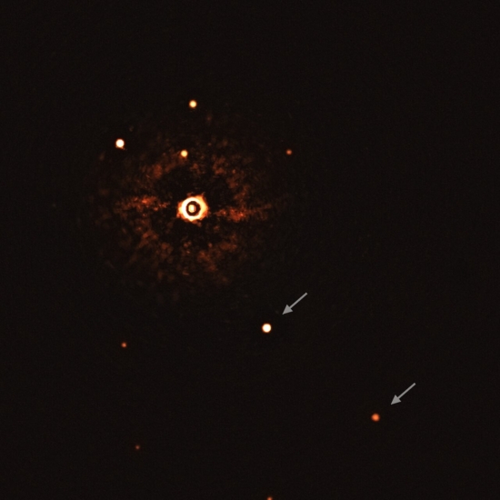
Image: This image, captured by the SPHERE instrument on ESO’s Very Large Telescope, shows the star TYC 8998-760-1 accompanied by two giant exoplanets, TYC 8998-760-1b and TYC 8998-760-1c. The two planets are visible as two bright dots in the centre (TYC 8998-760-1b) and bottom right (TYC 8998-760-1c) of the frame, noted by arrows. Other bright dots, which are background stars, are visible in the image as well. By taking different images at different times, the team were able to distinguish the planets from the background stars. The image was captured by blocking the light from the young, Sun-like star (top-left of centre) using a coronagraph, which allows for the fainter planets to be detected. The bright and dark rings we see on the star’s image are optical artefacts. Credit: ESO/Bohn et al.
Different forms of the same atom, isotopes vary in the number of neutrons housed in the nucleus, so that while carbon-12 has six neutrons to go along with its six protons, carbon-13 has seven neutrons and carbon-14 has eight. The distinctions are useful because while chemical properties remain largely the same, isotopes can be distinguished as they react to different conditions and are formed in different ways.
Zhang’s team drew on the distinction between carbon-13 and carbon-12 as marked by the way each absorbs radiation at slightly different colors, using ESO’s Spectrograph for Integral Field Observations in the Near Infrared (SINFONI), mounted on the Unit 3 instrument of the VLT. Expecting about one in 70 carbon atoms to be carbon-13, they found twice the number. The planet’s formation seems to be implicated, according to co-author Paul Mollière (Max Planck Institute for Astronomy, Heidelberg):
“The planet is more than one hundred and fifty times further away from its parent star than our Earth is from our Sun. At such a great distance, ices have possibly formed with more carbon-13, causing the higher fraction of this isotope in the planet’s atmosphere today.”
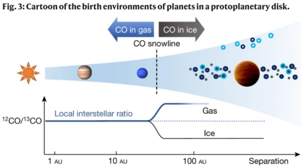
Image: This is Figure 3 from the paper. Caption: The two planets inside the CO snowline denote Jupiter and Neptune at their current locations, whereas TYC 8998 b is formed far outside this regime, where most carbon is expected to have been locked up in CO ice and formed the main reservoir of carbon in the planet. We postulate that this far outside the CO snowline, the ice was 13CO-rich or 13C-rich through carbon fractionation, resulting in the observed 13CO-rich atmosphere of the planet. A similar mechanism has been invoked to explain the trend in D/H within the Solar System. Future isotopologue measurements in exoplanet atmospheres can provide unique constraints on where, when and how planets are formed. Credit: Zhang et al.
The study of isotope abundance ratios has proven significant in studying not only interstellar chemistry and star formation but also the evolution of the Solar System. While its uses in analyzing exoplanet atmospheres are in their infancy, the hope is that future work on a range of exoplanets will offer clues to their formation.
The paper is Zhang et al., “The 13CO-rich atmosphere of a young accreting super-Jupiter,” Nature 595 (14 July 2021), 370-372. Abstract.
NEA Scout: Sail Mission to an Asteroid
Near-Earth Asteroid Scout (NEA Scout) is a CubeSat mission designed and developed at NASA’s Marshall Space Flight Center in Huntsville and the Jet Propulsion Laboratory in Pasadena. I’m always interested in miniaturization, allowing us to get more out of a given payload mass, but this CubeSat also demands attention because it is a solar sail, the trajectory of whose development has been a constant theme on Centauri Dreams.
And while NASA has launched solar sails before (NanoSail-D was deployed in 2010), NEA Scout moves the ball forward by going beyond sail demonstrator stage to performing scientific investigations of an asteroid. As Japan did with its IKAROS sail, the technology goes interplanetary. Les Johnson (MSFC) is principal technology investigator for the mission:
“NEA Scout will be America’s first interplanetary mission using solar sail propulsion. There have been several sail tests in Earth orbit, and we are now ready to show we can use this new type of spacecraft propulsion to go new places and perform important science. This type of propulsion is especially useful for small, lightweight spacecraft that cannot carry large amounts of conventional rocket propellant.”
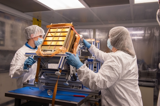
Image: Engineers prepare NEA Scout for integration and shipping at NASA’s Marshall Space Flight Center in Huntsville, Alabama. Credit: NASA.
The spacecraft, one of several secondary payloads, has been moved inside the Space Launch System (SLS) rocket that will take it into space on the Artemis 1 mission, an uncrewed test flight. Artemis 1 will be the first time the SLS and Orion spacecraft have flown together (the previous launch was via a Delta IV Heavy). NEA Scout, which will deploy after Orion separates, has been packaged and attached to an adapter ring connecting the SLS rocket and Orion.
Once separated from the launch vehicle, NEA Scout will deploy a thin aluminized polymer sail measuring 85 square meters (910 square feet). In terms of sail deployment, we can think of the mission as part of a continuum leading to Solar Cruiser, which will feature a sail 16 times larger when it launches in 2025. Deployment will be via stainless steel alloy booms. Near the Moon, the spacecraft will perform imaging instrument calibration and use cold gas thrusters to adjust its trajectory for a Near-Earth Asteroid. The solar sail will provide extended propulsion during the approximately two year cruise to destination. The final target asteroid has yet to be selected.
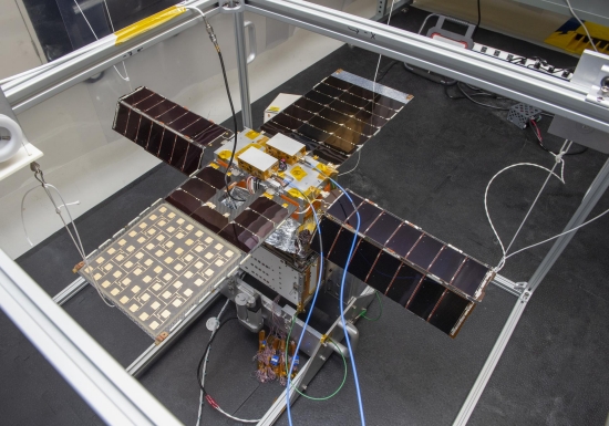
Image: NASA’s NEA Scout spacecraft in Gravity Off-load Fixture, System Test configuration at NASA’s Marshall Space Flight Center in Huntsville, AL. Credit: NASA.
The pace of innovation in miniaturization is heartening. I note this from a 2019 conference paper describing the final design and the challenges in perfecting the hardware (citation below):
The figurative explosion in CubeSat components for low earth orbital (LEO) missions proved that spacecraft components could be made small enough to accomplish missions with real and demanding science and engineering objectives. Unfortunately, these almost-off-the-shelf LEO components were not readily usable or extensible to the more demanding deep space environment. However, they served as an existence proof and allowed the NEA Scout spacecraft engineering team to innovate ways to reduce the size, mass, and cost of deep space spacecraft components and systems for use in a CubeSat form factor.
Image: Illustration of NEA Scout with the solar sail deployed as it flies by its asteroid destination. Credit: NASA.
At destination, NEA Scout is to perform a sail-enabled low-velocity flyby at less than 30 meters per second, with imaging down to less than 10 centimeters per pixel, which should enlarge our datasets on small asteroids, those measuring less than 100 meters across. Says principal science investigator Julie Castillo-Rogez (JPL):
“The images gathered by NEA Scout will provide critical information on the asteroid’s physical properties such as orbit, shape, volume, rotation, the dust and debris field surrounding it, plus its surface properties.”
The more we learn about small asteroids, the better, given our need to track trajectories and potentially change them if we ever find an object on course to a possible impact on Earth.
The presentation on NEA-Scout is Lockett et al., “Lessons Learned from the Flight Unit Testing of the Near Earth Asteroid Scout Flight System,” available here.
Europa: Below the Impact Zone
Yesterday we looked at the behavior of ice on Enceladus, a key to making long range plans for a lander there. But as we saw with Kira Olsen and team’s work, learning about the nature of ice on worlds with interior oceans has implications for other ice giant moons. This morning we look at the hellish surface environment of Europa, as high-energy radiation sleets down inside Jupiter’s magnetic field.
Europa’s surface radiation will complicate operations there and demand extensive shielding for any lander. But below the ice, that interior ocean should be shielded and warm enough to offer the possibility of life. With Europa Clipper on pace for a 2024 launch, we need to ask how the surface ice has been shaped and where we might find biosignatures that could have been churned up from below.

Tidal stresses on the ice leading to fracture are one way to force material up, but small impacts from above — debris in the Jovian system — also roil the surface. If we’re looking for potential biosignatures, we have to consider this surface churn and the effects of radiation upon what it produces. This is the subject of new work from a team led by Emily Costello (University of Hawai?i at Manoa), which has been studying the effects of electron radiation accelerated by Jupiter on complex molecules.
Image: The University of Hawai?i at Manoa’s Costello. Credit: UH Manoa.
The operative term in this paper, just published in Nature Astronomy, is impact gardening. The authors estimate through their modeling that the surface of Europa has been affected up to an average depth of 30 centimeters (about 12 inches). Over millions of years, the impacts add up even as surface material mixes with the subsurface, all bathed by radiation.
“If we hope to find pristine, chemical biosignatures, we will have to look below the zone where impacts have been gardening,” says Costello. “Chemical biosignatures in areas shallower than that zone may have been exposed to destructive radiation.”

Image: In this zoomed-in area (Figure 2) of Europa’s surface, an inset to Figure 1, a cliff runs across the middle of the image, revealing the interiors of the ridges leading up to it. The thin, bright layer at the top of the cliff is at least 20 to 40 feet (6 to 12 meters) thick. This thin surface layer, and possibly layers like it elsewhere over Europa’s surface, is where a process called “impact gardening” is thought to occur. Impact gardening is the small-scale mixing of the surface by space debris, such as asteroids and comets. Scientists are studying the cumulative effects of small impacts on Europa’s surface as NASA prepares to explore the moon with the upcoming Europa Clipper mission. New research and modeling estimate that the surface of Europa has been churned by small impacts to an average depth of about 12 inches (30 centimeters), within the layer of the surface that is visible here. Credit: NASA/JPL-Caltech.
The study looks not only at surface impacts but goes on to consider secondary impacts when debris returns to the surface after the initial strike. We learn there is a case for a particular zone on Europa — the moon’s mid- to high-latitudes — that would be less affected by radiation. In any case, a robotic lander may need to probe at least 30 centimeters down to find material unaffected by the ongoing impact gardening.
Rebecca Ghent (Planetary Science Institute, Tucson) is a co-author on the study:
“The work in this paper could provide guidance for design of instruments or missions seeking biomolecules; it also provides a framework for future investigation using higher-resolution images from upcoming missions, which would help to generate more precise estimates on the depth of gardening in various specific regions. The key parameters in this study are the impact flux and cratering rates. With better estimates of these parameters, and higher-resolution imaging resulting from upcoming missions, it will be possible to better predict the depths to which gardening has affected the shallow ice in specific regions.”
As a side note, I found when looking through Costello’s other papers that she and Ghent have done work on impact gardening at Ceres as well as Mercury and our own Moon. The paper on Ceres argues that the phenomenon is orders of magnitude less intense on Ceres than on the Moon, involving a much thinner regolith and leaving surface ice to be affected primarily by sublimation rather than impacts. It seems clear that our work on icy gas giant moons will need to take impact gardening into consideration, just as we monitor the movement of crustal ice.
The paper is Costello et al., “Impact gardening on Europa and repercussions for possible biosignatures,” Nature Astronomy 12 July 2021 (abstract). The paper on Ceres is Costello et al., “Impact Gardening on Ceres,” Geophysical Research Letters 11 April 2021 (abstract).

Follow with RSS or E-Mail
