Centauri Dreams
Imagining and Planning Interstellar Exploration
Beamer Technology for Reaching the Solar Gravity Focus Line
Alex Tolley’s essay on using beaming technology to reach the solar gravity focus (SGF) caught the eye of Jim Benford, who has been exploring the prospects for beamed sails for many years. Along with brother Greg, Jim did laboratory work at the Jet Propulsion Laboratory some 20 years ago to demonstrate the method, and in the years since has written extensively on the uses of beaming within the Solar System as well as on interstellar trajectories. But what kind of beam are we talking about? Benford, a plasma physicist and CEO of Microwave Sciences, has done recent work on a gravitational focus mission in connection with Breakthrough Starshot. He points to the maturity of microwave technology and the cost savings involved in using microwaves for a mission far faster than anything that has yet flown.
by James Benford

An intermediate destination for beamed energy interstellar probes, such as Starshot, is the Sun’s Inner Gravitational Focus (SGF). Alex Tolley suggests using Beamer technology for this mission. Gregory Matloff and I studied this approach in 2018 in work on the Starshot Project and published it [1]. This is a summary and update of that work.
The on-going Starshot technology development program will build a modular Beamer system that will incrementally achieve steadily higher launch speeds. As the Starshot technology develops, velocity regimes beyond anything available now will be attained. This will include flyby probes of the outer solar system planets and moons, exploration of the Kuiper belt objects and interstellar precursors to investigate beyond the heliopause. All these missions have the advantage of not requiring any deceleration as the objective is reached. Thus consideration of earlier missions and destinations nearer than the Centauri system is in order.
Here we consider a specific application of the basic Starshot concept, to fly a mission at 100 km/sec. We take sailcraft parameters from Parkin’s Starshot System Model, a thin-film circular photon sail with a mass of 4 grams, a payload of 1.5 grams, a diameter of 5 meters and a thickness of about 0.1 micron (0.2 g/m2, in the range of graphene) [2]. In order not to choose the system parameters arbitrarily, we use the Beamer cost optimization method developed by Benford [3], which minimizes the total system cost.
Why Cost Matters
The approach in our paper is to stipulate the key parameters; mass and velocity, then minimize the cost of the system. All other parameters, such as the sail diameter and, most importantly, the frequency of the Beamer are varied in order to minimize costs. Why does cost matter? These are very expensive systems: note that Starshot is designed/optimized to have a system cost below $10B. We showed SGF Beamer Systems can be in order of magnitude lower.
Economies of Scale
The costs include the decrease in unit cost of hardware with increasing production, economies of scale [3]. The components we’re modeling here, sources of microwave, mm-wave and laser beams, antennas and optics, must be produced in large quantities for the large scales of directed energy-driven sails. High-volume automated manufacturing would drive costs down.
Cost-Optimized Systems
Microwave Beamer cost is 580 M$. (Parameters are wavelength 0.03 m, frequency 10 GHz) parameters for 100 km/sec, 3 gram, 5-meter diameter sail, perfect reflectivity, 0.3m wavelength.) Microwave costs have reached true economies of scale and are now available in quantity at about 0.01 $/W and about 100 $/m2. Consequently, there is no need to extrapolate future microwave cost because present costs are low enough to use.
Millimeter-Wave Beamer cost is 2 B$. Thus far, millimeter-wave (wavelength 3mm, 100 GHz) devices at ~ 1 MW are available at $6/W and 10,000 $/m2. No large market has developed for millimeter-wave devices, so economies of scale have not been firmly established. We assume the learning curve of millimeter-wave tubes will be approximately that of similar tube devices, such as klystron, for which the learning curve is well established. At present the largest application for a megawatt-level millimeter-wave sources is the ITER fusion project, which requires hundreds of devices. An emerging near-term application for millimeter-wave technologies is for 5G Wi-Fi. Although the power levels will be low because of the short-range requirement, mass manufacture of millimeter-wave transmitters and apertures may enable substantial cost reductions to be realized in the next few decades.
Laser Beamer cost is >5.3 B$. Parkin estimates contemporary costs as at least $150/W and 1M $/m2. There are several options for the technology of the laser Beamer: from small mm-scale wafers at ~ 1 W power to larger ~500 W lasers with long coherence length (a key constraint in operating an array). Cost elements include emitters, optics and amplifiers. Lasers are being used for LIDAR in autonomous vehicles and at powers of 10-100 W, cost 100-$1000 $/W. At the higher figure, the Beamer would cost 23 B$!
The large number of sails needed to provide a useful image of an exoplanet means that we must take into consideration the cost of sails. Each sail will cost far less than the Beamer. We estimated the cost of such sails at ~1M$ each [1].
Technology Readiness and Feasibility
- State-of-the Art. Several practical factors favor microwave and millimeter waves over lasers, because they have practical advantages: Microwave equipment such as sources, anechoic rooms, antennas and diagnostics are commonly available than the emerging technology of high power lasers. That’s because microwave and millimeter wave sources, waveguide and supporting equipment, such as power supplies, are a developed industry. That means it is cheaper and faster to build systems. Lasers are developing fast, but at present are still expensive, and are produced in small numbers at slow rates.
- Efficiency. Microwaves are more efficient than lasers, typically 50-90%. Millimeter wave generation technologies now make it possible to generate wavelengths as short as 0.1 cm with relatively high efficiency (>40%). Laser efficiencies are ~40% now and have been slowly rising.
- Phased Arrays. Microwave phased arrays of transmitters and apertures are relatively easily done and are widely used, while phased arrays of laser beams, although possible in principle, subject to the coherence length constraint related above, are thus far little developed in practice. Work to date on laser phased arrays has been limited to small numbers of sources and modest power levels.
Desorption-Assisted Sail Missions
A different method that the JPL group has apparently not noticed is to use the desorption of various materials from the sail, ‘paints’, as it passes perihelion near the sun. That multiplies the utility of the solar sail technique substantially.
Thermal desorption consists in atoms, embedded in a substrate, that are liberated by heating, thus providing an additional thrust. Desorption can attain high specific impulse if low mass molecules or atoms are blown out of a lattice of material at high temperature.
Desorption of materials from hot sails in flight was observed in 2000 in microwave beam-driven carbon sail experiments I was conducting [4]. We found out that photon pressure could account for 3-30% of the observed acceleration, while the remainder came from desorption of embedded molecules.
After we understood what we were observing, my brother Gregory suggested it be used as a means of propulsion for sails [5,6]. The extraordinary potential of this sort of propulsion mechanism: if properly used, desorption could enhance thrust by orders of magnitude, shorten mission times.
Roman Kezerashvili and his fellow researchers have conducted detailed studies using desorption for solar sail missions to obtain high velocities [7]. Kezerashvili recently published a review article about this [8].
Conclusion
Therefore if we are to send probes to the SGF in this era, my calculations show that the lowest cost Beamer will be a microwave system. This will enable a transportation system within the Solar System that could be realized far sooner than laser arrays.
A solar sail augmented by desorption propulsion may give better performance for solar sail missions to the Sun’s Gravitational Focus.
If exoplanet imaging from the SGF is to be done soon, microwave or millimeter-wave beam systems could be built with existing technology now. Developing the phased array laser Beamer and driving the cost down to where larger arrays can be afforded will take decades. Similarly, it will take decades to conduct the test demonstrations required to prove the solar sail approach in the inner solar system. Advocates of both approaches should acknowledge these necessary timescales.
References
1. James Benford & Gregory Matloff, “Intermediate Beamers for Starshot: Probes to the Sun’s Inner Gravity Focus”, JBIS 72, 51-55, 2019.
2. Kevin Parkin, “The Breakthrough Starshot System Model”, Acta Astronautica 152 370, 2018.
3. J. Benford, “Starship Sails Propelled by Cost-Optimized Directed Energy”, JBIS 66 85, 2013.
4. James Benford et al., Flight and Spin of Microwave-Driven Sails, Final Report, Contract Number NAS8-99135, 2000. See also short version: “Flight and Spin of Microwave-driven Sails: First Experiments”, James Benford, Proc. Pulsed Power Plasma Science 2001, IEEE 01CH37251, 548, 2001.
5. Gregory Benford & James Benford “Desorption Assisted SunDiver Missions”, AIP Conf. Proc. 608, 462-469, 2002.
6. Gregory Benford, & James Benford, “Acceleration of Sails by Thermal Desorption of Coatings”, Acta Astronautica 56, 593-599, 2005.
7. Elena Ancona, Roman Ya. Kezerashvili, & Gregory L. Matloff, “Exploring the Kuiper Belt with sun-diving solar sails”, Acta Astronautica 160, 601-605 2019.
8. Elena Ancona & Roman Ya. Kezerashvili, “Extrasolar Space Exploration by a Solar Sail Accelerated via Thermal Desorption Of Coating”, Advances in Space Research 63 2021-2034, 2019.

A Beamed Sail to the Sun’s Gravity Focus
Our recent discussions about Claudio Maccone’s FOCAL mission to the Sun’s gravitational focus, and the ongoing work at the Jet Propulsion Laboratory for NASA’s Innovative Advanced Concepts office, have had Alex Tolley thinking about alternative scenarios. Yes, a spacecraft moving along the focal line extending from the solar gravitational lens (SGL) would be capable of extraordinary imaging, and could serve as a communications relay for interstellar probes, but that tricky Sundiver maneuver suggested by Slava Turyshev and team in their ‘string of pearls’ concept puts huge demands on sail materials. Moreover, we’d ideally like to be able to slow the craft as it moves along the focus, to allow maximum time for observations. To achieve both fast transit and maneuverability at the gravitational focus, Alex advocates beamed propulsion, a method whose advantages and consequences are discussed below. Synergies with the ongoing Breakthrough Starshot effort are apparent.
by Alex Tolley
The huge increase in discovered exoplanets, many in the habitable zones (HZ) of their stars, has increased the push to determine if life exists on any of these worlds. With even our best telescopes, light from these worlds is just a single pixel in extent, which allows spectrographic analysis for biosignatures and techno-signatures. However, a 2D image of an exoplanet would answer many more questions about these worlds. The image makes a lot of difference both to scientists and the public. The astronomy books of my youth showed the moons of the gas giants as points of light, and Pluto was just a star-like object. As late as 2010, the Hubble telescope could only manage a crude blurry image of Pluto showing some light and dark regions. The New Horizon probe flyby with high-resolution images changed our view of the Pluto-Charon binary.
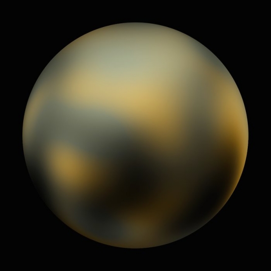
Image: Hubble 1200×1200 pixel image of Pluto in February 2010.
To acquire a megapixel image of even a nearby exoplanet would require a telescope of tens of kilometers in diameter to collect the light of the planet while masking out the far more intense light of its star. A possible solution was proposed by Claudio Maccone, with his proposed FOCAL mission to use our sun’s gravity to focus distant light rays on a telescope [5]. While there are technical issues still to be resolved in how to form a low noise 2D image of 10,000 (100 x 100) to 1 million (1000 x 1000) pixels, the big question is:
“How do we get there in a short enough time for a project , and how do we best collect the data to make the image?”
The Sundiver Problem
The solar gravitational focus (SGF) is a line extending from about 550 AU to infinity. The focus starts out in interstellar space. For comparison, Voyager 1 launched over 40 years ago and has just passed through the heliopause of our sun and into interstellar space. It is only ¼ of the way to the SGF. It will not reach the focus for another 120 years. Clearly, we need a much faster way to reach the focus so that scientists and engineers can reasonably engage in a realistic mission, rather than taking the generations that were required to build a cathedral.
At this point, we can rule out most propulsion technologies, even using gravity assists. The most promising is a solar sail, and as I will argue, a sail augmented with a beam.
The authors of the recent NIAC II report [1, 6] opt for a pure solar sail. They propose a mission that could reach the SGF within a reasonable 25 years using a very advanced solar sail and leveraging a ‘sundiver’ trajectory. This sail could achieve a velocity of 25 AU/yr (about 125 km/s), of which most of that velocity is achieved quickly as the sail leaves perihelion. When I say ‘advanced,’ the mission needs a sail that has an areal density of less than 10 g/m2, and possibly 1 g/m2. Note that this density is not just the sail material, but must include the probe structure, payload, and any auxiliary equipment, such as communications, maneuvering thrusters, etc.
To put this in perspective, the Planetary Society’s CubeSat LightSail has an areal density of about 143 g/m2, a similar density as the upcoming NEA Scout probe. The target areal density of the Breakthrough Starshot beamed sail is 1.4 g/m2, achieved by having just a chip-sized payload on the sail of just 1 m2 [4].
Without such low areal densities, 2 to 4 orders of magnitude lower than currently achieved, there is no hope of reaching the needed velocities. The sail craft must also do a sundiver maneuver to gain maximum thrust at perihelion. Maximum velocity is achieved by the orbit of Saturn. How close the sail can approach the sun depends on the sail materials. To get both the very low sail mass to achieve the needed areal density, and approach the sun to within 0.1 AU (15 million km) requires a strong, low-density material with a high melting point, such as a ceramic.
If such a solar sail is achievable, then the craft with its telescope payload will continue on into interstellar space along the focal line.
While the focal line continues to infinity, is there an optimum “sweet spot” to image the target? Maccone states that although complex, the best position might be fairly close to the 550 AU start of the SGF [1]. If that is correct, it is suboptimal to allow the telescope to continue traveling rapidly away from that position.
The NIAC authors solve this rather cleverly: launch a series of sails, a year apart, forming a “string of pearls” separated by 25 AU, so that each probe stays within 25 AU of the start of the SGF at 550 AU before handing off the data collection to the next probe, or even contributing to the collection of other data as it journeys on into interstellar space.
This solution has several disadvantages, not the least of which is the need to ensure that each sail can align independently and correctly with the target.
Therefore, ideally, one would want the sailcraft and its telescope to effectively stop at the best distance just beyond 550 AU. This has several advantages:
- The focus remains unchanged – reducing issues with image deconvolution
- The required coronagraph to isolate the Einstein ring of light is fixed in dimension and position.
- The tracking of both the target star’s position and the exoplanet in its orbit is simplified as the distance to track relative motion increases as the distance from the sun increases.
- Only one imaging telescope is needed, as well as the auxiliary equipment. The scale economies of building and flying multiple sails can be used to image multiple targets instead of just one.
- Data collection can be as long as desired, not fixed for the number of sails sent, allowing better images to be produced, as well as longer-term observations of the target for other purposes. If the payload includes a receiver for a communication bridge to a probe orbiting an exoplanet, the communication link can be established for as long as needed, perhaps many decades.
Using sail material that is off-the-shelf, how could we achieve such a mission?
The Benefits of Beamed Propulsion
My proposed solution is to use a beamed sail. The beam would most likely be a phased laser array located on Earth with the capability of pushing a sail in all but the highest latitudes. This is the type of power source that is being studied by the Breakthrough StarShot team. Because the sail need not achieve the fractional c velocities needed for interstellar flight, the size of the sail, payload, and beam intensity on the sail can be matched to the materials and payload requirements. Ideally, the sail velocity would exceed that of 25 AU/yr to shorten the flight time, but no longer restricted to the high-performance sundiver mission needed to reach that velocity. There is also no need to tolerate high temperatures at perihelion, although this will also depend on the laser power and duration.
Moreover, there is a way to stop a beamed sail, which was suggested by Robert Forward [7]. Figure 1 below shows a schematic of the concept for this deceleration maneuver.
The sail would separate into 2 parts with the larger part focussing the beam on the smaller sail to decelerate it. This was proposed by Forward as a way to decelerate a sail and its payload on arriving at its desired destination. The same approach could be used to decelerate a beamed sail when it reaches the 550 AU minimum focus position. When “stopped”, the sail would deploy its imager/receiver.
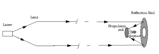
Image: Schematic of the round-trip interstellar lightsail concept proposed by Forward (not to scale), shown during the deceleration phase. Credit: Geoffrey Landis [2].
The relative sizes of the two sails will depend on the achievable laser strength on the sail over the deceleration distance that ends around 550 AU, and on how well the reflected beam can be targeted to the sail with the payload. The aim is to slow the smaller sail with the telescope payload down towards a dead stop, although any low velocity, like that of Voyager 1, is adequate to ensure a long data collection period and minimal changes to the required maneuvering to track the star and planet. Pointing the laser at the sail will require relatively simple position prediction up to about 160 hours in the future based on the most recent time-stamped location received from the craft. [160 hours is 2x the light travel time to 550 AU; signal sent from the craft that reaches earth 80 hours later and the next 80 hours for the beam to reach the sail.]
The slow movement of the stars relative to the sun will still require some traversal across the focus to track this motion and ensure the craft stays within the best position to receive the communication or visual image. For example, Proxima moves about 3.85 arcseconds per year across the heavens. At 550 AU, this implies that to keep the sun in line with Proxima, the craft must travel a modest 50 m/s to maintain position.
One issue not so far mentioned is the position of the stellar target in the sky. Unlike most of our planetary missions to date, where the planets fairly closely aligned with the ecliptic, the target stars for an SGL mission are spread out over the celestial sphere. For example, Alpha Centauri is in the southern sky with a declination of over -62 degrees. The TRAPPIST 1 planetary system, about 40 ly away, with some possibly very interesting exoplanets in close proximity for imaging, is about -5 degrees of declination when observed from Earth. The sail craft must travel in the opposite direction so that the target is directly behind the sun, so that for Proxima the telescope must be positioned with a declination of over +62 degrees and the appropriate 180 degrees offset to right ascension.
Each sail craft can only image one target star at a time, although if that star has several planets, all these planets may be imaged over time. The stars are far too separated over the celestial sphere for any reasonable time to navigate between them. For the 30 pc (100 ly) volume, the 15,500+ FGK stars would be separated by about 60 AU on average. Therefore each sailcraft could only image one star system. This would therefore require considerable care in selection. However, given the laser infrastructure and the scale economy of manufacturing the sail craft, it might well make sense to send many craft out to their SGF positions.
The benefit of a FOCAL mission to acquire relatively high resolution images of exoplanets far beyond any single telescope we can envision today is offset by the demands of reaching the gravitational focal line starting at 550 AU. Once there, ideally, the craft should not continue its outbound journey. To achieve this, a beamed sail that can decelerate its payload is proposed.
References
1. Gilster, P. (2020) JPL Work on a Gravitational Lensing Mission, https://www.centauri-dreams.org/2020/12/16/jpl-work-on-a-gravitational-lensing-mission/
2. Landis, G (1989). Optics and Materials Considerations for a Laser-propelled Lightsail” http://www.geoffreylandis.com/lightsail/Lightsail89.html
3. Vulpetti, G., Johnson, L., & Matloff, G. L. (2008). Solar sails: A novel approach to interplanetary travel. New York: Copernicus Books.
4. Montgomery, E, Johnson, L, (2017) Solar Sail Propulsion: A Roadmap from Today’s Technology to Interstellar Sailships. Presentation to Foundations of Interstellar Studies Workshop, New York City College of Technology, Brooklyn, NY
5. Maccone, C. (2009) Deep Space Flight And Communications: Exploiting The Sun As A Gravitational Lens (Springer Praxis Books / Astronautical Engineering)
6. Turyshev et al. (2020), “Direct Multipixel Imaging and Spectroscopy of an Exoplanet with a Solar Gravity Lens Mission.” Final Report. NASA Innovative Advanced Concepts Phase II
7. Forward, R (1984) “Roundtrip interstellar travel using laser-pushed lightsails,” American Institute of Aeronautics and Astronautics, v21 No.2, pp 187-195
A Holiday Thought Looking Ahead
I want to send along best wishes for the season to all of you. Centauri Dreams started as a book and became a study guide for me as I tried to keep up with ongoing developments in deep space research. But turning the site into a community, which I did in 2005 by adding comments, has been what really made it go, as I’ve continued to learn from the discussions between readers, finding new resources and different insights I would never have achieved on my own. So thank all of you for this continuing gift, and may this holiday season be the prelude to great discoveries ahead.
Stellar Flares as an Aid to Life Detection
The interesting transient associated with Proxima Centauri and monitored by Breakthrough Listen reminds us of a key fact about red dwarf stars and the planets around them. Such stars, especially in their youth, are prone to high flare activity, meaning violent, unpredictable emissions that can deplete atmospheric gases like ozone. Even if the atmosphere survives strong stellar winds, the loss of ozone can lead to high levels of ultraviolet radiation reaching the surface and compromising any life there.
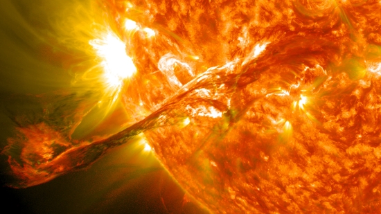
That stellar flares can be dramatic is captured in the image below, showing a filament eruption from the Sun and accompanying solar flares (credit: NASA/GSFC/SDO). As striking as the image is, it depicts activity on an older star less prone to strong flare activity than younger, smaller stars. We’re also fortunate in having the shield offered by Earth’s magnetic field, which can deflect the worst of the solar wind. Our G-class Sun lets us orbit at a comfortable distance, but planets in the habitable zones of M-class dwarfs are in tight orbits. Proxima Centauri b, for example, orbits its primary in a scant 11 days at a distance of 0.0485 AU.
This may or may not be a deal-breaker for life, given evolutionary change that may force adaptations we can only imagine, but it certainly creates stark conditions for its formation. Even so, such activity may also provide us with opportunities when it comes to observing biosignatures. This morning I learned about a study from Northwestern University that takes a close look at stellar flares and the evolution of planetary atmospheres. We learn that flare activity can create atmospheric changes that actually make certain biosignatures more detectable.
Northwestern’s Howard Chen is lead author on the study:
“We compared the atmospheric chemistry of planets experiencing frequent flares with planets experiencing no flares. The long-term atmospheric chemistry is very different. Continuous flares actually drive a planet’s atmospheric composition into a new chemical equilibrium.”
What the Northwestern team has done is to combine a suite of three-dimensional coupled chemistry-climate model simulations with observed flare activity from a variety of stars. The scientists examined planet scenarios with varying rotation period, magnetic field strength and flare frequency, showing that recurring flares drive the atmospheres of planets around both K- and M-class stars “into chemical equilibria that substantially deviate from their pre-flare regimes, whereas the atmospheres of G dwarf planets quickly return to their baseline states.”
We should be able to use this fact to our advantage. Flares may help us see otherwise undetectable atmospheric components like nitrogen dioxide, nitrous oxide and nitric acid, which the paper describes as “bio-indicating chemical species.” Nearby red dwarfs, already useful because of their transit depth (a big planet passing in front of a small star is readily seen) now offer new ways to hunt biosignatures as next-generation space telescopes come online.
The study examines planets within the habitable zones of M- and K-class stars, where the habitable zones are smaller and the stellar activity more frequent. Tidally locked planets in this setting, with one face turned toward their star at all times, may lack the magnetic fields needed to deflect their stellar winds. The researchers used flare data from TESS, NASA’s Transiting Exoplanet Survey Satellite, in adjusting their simulations. From the paper:
For all scenarios, we find that flaring produces the largest magnitude alteration in nitrous oxide (N2O), a biosignature… Both HNO3 and H2Ov mixing ratios are enhanced on average by two to three orders of magnitude and the enhancements are maintained with repeated flaring in the K- and M-star planet scenarios… In contrast, CH4 experiences stronger removal via reaction with ion-derived OH during flaring, leading to lower temporal-mean CH4 mixing ratios (not shown). These results suggest that although biosignatures such as CH4 are vulnerable to destruction during periods of strong flaring, bio-indicating ‘beacon of life’ species could be prominently highlighted.

Image: An artistic rendering of a series of powerful stellar flares. Credit: NASA’s Goddard Space Flight Center/S. Wiessinger.
Published in Nature Astronomy, the research includes contributions from researchers at the University of Colorado at Boulder, the University of Chicago, Massachusetts Institute of Technology and NASA’s Nexus for Exoplanet System Science (NExSS).
Notice that we are increasingly studying exoplanet atmospheres in relation to space weather in the host star’s vicinity. Understanding how the signatures of chemical components vary with stellar activity like coronal mass ejections and flares — and in particular what the observational consequences may be — will help us shape the observing campaigns of future instruments, with consequences for detecting biosignatures.
The paper is Chen et al., “Persistence of flare-driven atmospheric chemistry on rocky habitable zone worlds,” Nature Astronomy 21 December 2020 (abstract).
A Transient at Proxima Centauri?
I see there’s now a Wikipedia page for BLC-1, the intriguing SETI detection made by Breakthrough Listen at the Parkes Observatory in Australia. The dataset in which the signal, found at 982 MHz, turned up comes from observations made in April and May of 2019, and it’s good to know that Breakthrough is working up two papers on the signal and subsequent analysis, given that the public face of the detection was originally in the form of a story leaked to the British newspaper The Guardian before the backup research was available.
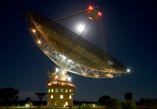
Image: CSIRO’s Parkes radio telescope in New South Wales, Australia. Credit: Shaun Amy.
The first thing to say about BLC-1 is that the acronym stands for Breakthrough Listen Candidate 1, marking the first time a signal has made it through to actual ‘candidate’ status after five years of observations, which is itself noteworthy given the intensity of the effort.
The second thing is that this is a transient, meaning it’s short-lived, and it hasn’t repeated. That gets us into tricky territory, for the SETI effort has detected numerous transients over the years, and the lack of repetition has made confirmation of their origin difficult if not impossible. The most famous is the Wow! signal detected at Ohio State in 1977, a signal that continues to inspire research, as we’re about to see in a new paper that considers some of its more unusual aspects. But more on that within a few weeks.
The BLC-1 transient may or may not be from Proxima Centauri, which is the reason for the question mark in the title. I say that because we can’t yet rule out terrestrial interference of some kind. But there are transients and there are transients, and this one does raise the eyebrows. Back in April of last year, Breakthrough was working with the Parkes instrument to study the flare activity at Proxima Centauri, a significant issue as we consider questions of habitability on planets around red dwarf stars because flares can compromise a planetary atmosphere.
The detection of BLC-1 within the Proxima data is credited to Shane Smith, an undergraduate at Hillsdale College (Michigan) working as an intern within the Breakthrough Listen project. Smith’s claim to fame should be air-tight if BLC-1 turns out to be the real deal.
We do know that the signal is narrow in bandwidth and vanished when the instrument looked away from Proxima Centauri. It contains no sign of modulation. The signal also showed some drift in frequency, which would be consistent with a source in motion; i.e., a planet orbiting a star. The intriguing habitable zone planet Proxima b has commanded attention as being an Earth-mass planet around the nearest star, and is often mentioned as a possible target for Breakthrough Starshot probes. But even the matter of drift is unusual, as Lee Billings and Jonathan O’Callaghan point out in an article in which they interviewed Breakthrough’s Sofia Sheikh (Penn State):
…the signal “drifts,” meaning that it appears to be changing very slightly in frequency—an effect that could be due to the motion of our planet, or of a moving extraterrestrial source such as a transmitter on the surface of one of Proxima Centauri’s worlds. But the drift is the reverse of what one would naively expect for a signal originating from a world twirling around our sun’s nearest neighboring star. “We would expect the signal to be going down in frequency like a trombone,” Sheikh says. “What we see instead is like a slide whistle—the frequency goes up.”
We’ve come a long way since November of 1967, when Jocelyn Bell Burnell discovered PSR B1919+21, the first radio pulsar, which was jokingly named LGM-1 (Little Green Men 1) by its discoverers. And why not? The signal seemed tight and remarkably regular.
While SETI has become far more visible since those days, we’ve seen how nature can mimic technology, but we’ve also learned that RFI – radio frequency interference – ranging from nearby transmitters to malfunctioning electronics, can get into the mix. Parkes had its ‘peryton’ bursts not so long ago, but they were traced back to problems with a nearby microwave oven.
A note on Y Combinator Hacker News last night (thanks for the tip, Steven Ward) points out that 982.000 MHz, for example, is also the wavelength of the Intel Stratix 10 FPGA, a field programmable gate array used for prototyping application-specific integrated circuits (ASICs). Several other hardware components listed there are also operating at this wavelength, a fact that Breakthrough’s analysts will doubtless be taking into account as they go through all the options for pinning this detection to terrestrial sources of RFI.
So we come back to the issue of transients and repetition. Thus far Breakthrough has subjected the BLC-1 signal to exhaustive analysis and no RFI has yet been identified. The work continues, valuable in and of itself because if this signal does turn out to be RFI, it will provide a way to fine-tune the existing Breakthrough algorithms to filter out such signals in the future.
And if we can’t find a plausible source of RFI? That would be interesting, to say the least, and we may be left with something like the Wow! signal, an intriguing but non-repeating source. I think we can say this: If it actually turns out that BLC-1 is the signature of an alien civilization, then we’ll be tempted to throw out the Fermi paradox (‘where are they?’), but also re-calibrate all our thinking about civilizations in the galaxy. After all, wouldn’t finding one around the star closest to the Sun imply we’re going to find them in great numbers almost wherever we look?
Maybe not. Who is it who said ‘the thing about aliens is that they’re alien?’ Meanwhile, we keep an eye on Proxima Centauri to see if this thing repeats.
JPL Work on a Gravitational Lensing Mission
Seeing oceans, continents and seasonal changes on an exoplanet pushes conventional optical instruments well beyond their limits, which is why NASA is exploring the Sun’s gravitational lens as a mission target in what is now the third phase of a study at NIAC (NASA Innovative Advanced Concepts). All of this builds upon the impressive achievements of Claudio Maccone that we’ve recently discussed. Led by Slava Turyshev, the NIAC effort takes advantage of light amplification of 1011 and angular resolutions that dwarf what the largest instruments in our catalog can deliver, showing what the right kind of space mission can do.
We’re going to track the Phase III work with great interest, but let’s look back at what the earlier studies have accomplished along the way. Specifically, I’m interested in mission architectures, even as the NASA effort at the Jet Propulsion Laboratory continues to consider the issues surrounding untangling an optical image from the Einstein ring around the Sun. Turyshev and team’s work thus far argues for the feasibility of such imaging, and as we begin Phase III, sees viewing an exoplanet image with a 25-kilometer surface resolution as a workable prospect.
But how to deliver a meter-class telescope to a staggeringly distant 550 AU? Consider that Voyager 1, launched in 1977, is now 152 AU out, with Voyager 2 at 126 AU. New Horizons is coming up on 50 AU from the Earth. We have to do better, and one way is to re-imagine how such a mission would be achieved through advances in key technologies and procedures.
Here we turn to mission enablers like solar sails, artificial intelligence and nano-satellites. We can even bring formation flying into a multi-spacecraft mix. A technology demonstration mission drawing on the NIAC work could fly within four years if we decide to fund it, pointing to a full-scale mission to the gravitational focus launched a decade later. Travel time is estimated at 20 years.
These are impressive numbers indeed, and I want to look at how Turyshev and team achieve them, but bear in mind that in parsing the Phase II report, we’re not studying a fixed mission proposal. This is a highly detailed research report that tackles every aspect of a gravitational lens mission, with multiple solutions examined from a variety of perspectives. One thing it emphatically brings home is how much research is needed in areas like sail materials and instrumentation for untangling lensed images. Directions for such research are sharply defined by the analysis, which will materially aid our progress moving into the Phase III effort.

Image: A meter-class telescope with a coronagraph to block solar light, placed in the strong interference region of the solar gravitational lens (SGL), is capable of imaging an exoplanet at a distance of up to 30 parsecs with a few 10 km-scale resolution on its surface. The picture shows results of a simulation of the effects of the SGL on an Earth-like exoplanet image. Left: original RGB color image with (1024×1024) pixels; center: image blurred by the SGL, sampled at an SNR of ~103 per color channel, or overall SNR of 3×10³; right: the result of image deconvolution. Credit: Turyshev et al.
Modes of Propulsion
A mission to the Sun’s gravity lens need not be conceived as a single spacecraft. Turyshev relies on spacecraft of less than 100 kg (smallsats, in the report’s terminology) using solar sails, working together and produced in numbers that will enable the study of multiple targets.
The propulsive technique is a ‘Sundiver’ maneuver in which each smallsat spirals in toward perihelion in the range of 0.1 to 0.25 AU, achieving 15-25 AU per year exit velocity, which gets us to the gravity lensing region in less than 25 years. The sails are eventually ejected to reduce weight, and onboard propulsion (the study favors solar thermal) is available at cruise. The craft would enter the interstellar medium in 7 years as compared to Voyager’s 40, making the journey to the lens in a timeframe 2.5 times longer than what it took to get New Horizons to Pluto.
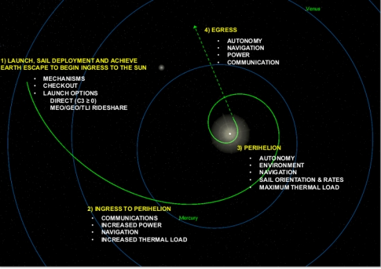
Image: Sailcraft example trajectory toward the Solar Gravity Lens. Credit: Turyshev et al.
The hybrid propulsion concept is necessary, and not just during cruise, because once in the focal lensing region, the spacecraft will need either chemical or electrical propulsion for navigation corrections and for operations and maintenance. Let’s pause on that point for a moment — Alex Tolley and I have been discussing this, and it shows up in the comments to the previous post. What Alex is interested in is whether there is in fact a ‘sweet spot’ where the problem of interference from the solar corona is maximally reduced compared to the loss of signal strength with distance. If there is, how do we maximize our stay in it?
Recall that while the focal line goes to infinity, the signal gain for FOCAL is proportional to the distance. A closer position gives you stronger signal intensity. Our craft will not only need to make course corrections as needed to keep on line with the target star, but may slow using onboard propulsion to remain in this maximally effective area longer. I ran this past Claudio Maccone, who responded that simulations on these matters are needed and will doubtless be part of the Phase II analysis. He has tackled the problem in some detail already:
“For instance: we do NOT have any reliable mathematical model of the Solar Corona, since the Corona keeps changing in an unpredictable way all the time.
“In my 2009 book I devoted the whole Chapters 8 and 9 to use THREE different Coronal Models just to find HOW MUCH the TRUE FOCUS is PUSHED beyond 550 AU because of the DIVERGENT LENS EFFECT created by the electrons in the lowest level of the Corona. For instance, if the frequency of the electromagnetic waves is the Peak Frequency of the Planckian CMB, then I found that the TRUE FOCUS is 763 AU Away from the Sun, rather than just 550 AU.
“My bottom-line suggestion is to let FOCAL observe HIGH Frequencies, like 160 GHz, that are NOT pushing the true focus too much beyond 550 AU.”
Where we make our best observations and how we keep our spacecraft in position are questions that highlight the need for the onboard propulsion assumed by the Phase II study.
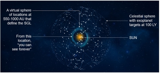
Image: Our stellar neighborhood with notional targets. Credit: Turyshev et al.
For maximum velocity in the maneuver at the Sun, as close a perihelion as possible is demanded, which calls for a sailcraft design that can withstand the high levels of heat and radiation. That in turn points to the needed laboratory and flight testing of sail materials proposed for further study in the NIAC work. Let me quote from the report on this:
Interplanetary smallsats are still to be developed – the recent success of MarCO brings them perhaps to TRL 7. Solar sails have now flown – IKAROS and LightSail-2 already mentioned, and NASA is preparing to fly NEA-Scout. Scaling sails to be thinner and using materials to withstand higher temperatures near the Sun remains to be done. As mentioned above, we propose to do this in a technology test flight to the aforementioned 0.3 AU with an exit velocity ~6 AU/year. This would still be the fastest spacecraft ever flown.
The report goes on to analyze a technology demonstration mission that could be done within a few years at a cost less than $40 million, using a ‘rideshare’ launch to approximately GEO.
String of Pearls
The mission concept calls for an array of optical telescopes to be launched to the gravity lensing region. I’ll adopt the Turyshev acronym of SGL for this — Solar Gravity Lens. The thinking is that multiple small satellites can be launched in a ‘string of pearls’ architecture, where each ‘pearl’ is an ensemble of smallsats, with multiple such ensembles periodically launched. A series of these pearls, multiple smallsats operating interdependently using AI technologies, provides communications relays, observational redundancy and data management for the mission. From the report:
By launching these pearls on an approximately annual basis, we create the “string”, with pearls spaced along the string some 20-25 AU apart throughout the timeline of the mission. So that later pearls have the opportunity to incorporate the latest advancements in technology for improved capability, reliability, and/or reductions in size/weigh/power which could translate to further cost savings.
In other words, rather than being a one-off mission in which a single spacecraft studies a single target, the SGL study conceives of a flexible investigation of multiple exoplanetary systems, with ‘strings of pearls’ launched toward a variety of areas within the focus within which exoplanet targets can be observed. Whereas the Phase I NIAC study analyzed instrument and mission requirements and demonstrated the feasibility of imaging, the Phase II study refines the mission architecture and makes the case that a gravity lens mission, while challenging, is possible with technologies that are already available or have reached a high degree of maturity.
Notice the unusual solar sail design — called SunVane — that was originally developed at the space technology company L’Garde. Here we’re looking at a sail design based on square panels aligned along a truss to provide the needed sail area. In the Phase II study, the craft would achieve 25 AU/year, reaching 600 AU in ~26 years (allowing two years for inner system approach to the Sun). [Note: I’ve replaced the earlier SunVane image with this latest concept, as passed along by Xplore’s Darren Garber. Xplore contributed the design for the demonstration mission’s solar sail].
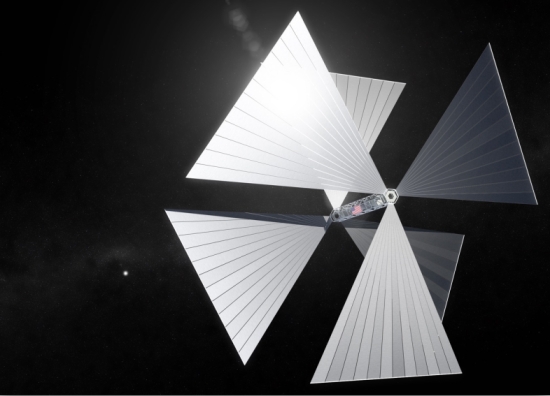
Image: The SunVane concept. Credit: Darren D. Garber (Xplore, Inc).
The report examines a sail area of 45,000 m2, equivalent to a ~212×212 m2 sail, with spacecraft components to be configured along the truss. Deployment issues are minimal with the SunVane design. The vanes are kept aligned edge-on to the Sun as the craft approaches perihelion, then directed face-on to promote maximum acceleration.
We have to learn how to adjust parameters for the sail to allow the highest possible velocity, with areal density A/m being critical — here A stands for the area in square meters of the sail, with m as the total mass of the sailcraft in kilograms (this includes spacecraft plus sail). Sail materials and their temperature properties will be crucial in determining the perihelion distance that can be achieved. This calls for laboratory and flight testing of sail material as part of the continuing research moving into the Phase III study and beyond. Sail size is a key issue:
The challenge for design of a solar sail is managing its size – large dimensions lead to unstable dynamics and difficult deployment. In this study we have consider[ed] a range of smallsat masses (<100 kg) and some of the tradeoffs of sail materials (defining perihelion distance) and sail area (defining the A/m and hence the exit velocity…). As an example, for the SGLF mission, consider perihelion distance of 0.1 AU (20Rsun) and A/m=900 m2/kg; the exit velocity would be 25 AU/year, reaching 600 AU in ~26 years (allowing 2 years for inner solar system approach to the Sun). The resulting sail area is 45,000 m2, equivalent to a ~212×212 m2 sail.
The size of that number provokes the decision to explore the SunVane concept, which distributes sail area in a way that allows spacecraft components to be placed along the truss instead of being confined to the sail’s center of gravity, and which has the added benefit of high maneuverability. A low-cost near-term test flight is proposed with testing of sail material and control, closing to a perihelion in the range of 0.3 AU, with an escape velocity from the Solar System of 6-7 AU per year. Several such spacecraft would enable a test of swarm architectures.
Thus the concept: Multiple spacecraft would be launched together as an ensemble — the ‘pearl’ — using solar sails deployed on each and navigating through the Deep Space Network, with the spacecraft maintaining a separation on the order of 15,000 km as they pass through perihelion. Such ensembles are periodically launched, acting interdependently in ways that would maximize flexibility while reducing risk from a single catastrophic failure and lowering mission cost. We wind up with a system that would enable investigations of multiple extrasolar systems.
I haven’t had time to get into such issues as communications and power for the individual smallsats, or data processing and AI, all matters that are covered in the report, nor have I looked in as much detail as I would have liked at the sail arrays, envisioned through SunVane as on the order of 16 vanes of 103 m2, allowing the area necessary in a configuration the report considers realistic. This is a lengthy, rich document, and I commend it to those wanting to dig further into all these matters.
The report is Turyshev et al., “Direct Multipixel Imaging and Spectroscopy of an Exoplanet with a Solar Gravity Lens Mission,” Final Report NASA Innovative Advanced Concepts Phase II (full text).

Follow with RSS or E-Mail
