Part II: Sherlock Holmes and the Case of the Spherical Lens: Reflections on a Gravity Lens Telescope

by Paul Gilster | Apr 28, 2023 | Uncategorized | 17 Comments

Aerospace engineer Wes Kelly continues his investigations into gravitational lensing with a deep dive into what it will take to use the phenomenon to construct a close-up image of an exoplanet. For continuity, he leads off with the last few paragraphs of Part I, which then segue into the practicalities of flying a mission like JPL's Solar Gravitational Lens concept, and the difficulties of extracting a workable image from the maze of lensed photons. The bending of light in a gravitational field may offer our best chance to see surface features like continents and seasonal change on a world around another star. The question to be resolved: Just how does General Relativity make this possible? by Wes Kelly Conclusion of Part I At this point, having one’s hands on an all-around deflection angle for light at the edges of a “spherical lens” of about 700,000 kilometers radius (or b equal to the radius of the sun rS), if it were an objective lens of a corresponding telescope, what would be...

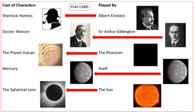
Sherlock Holmes and the Case of the Spherical Lens: Reflections on a Gravity Lens Telescope (Part I)

by Paul Gilster | Apr 25, 2023 | Exoplanetary Science | 16 Comments

A growing interest in JPL's Solar Gravitational Lens mission here takes Wes Kelly on an odyssey into the past. A long-time Centauri Dreams contributor, Wes looks at the discovery of gravitational lensing, which takes us back not only to Einstein but to a putative planet that never existed. Part II of the essay, which will run in a few days, will treat the thorny issues lensing presents as we consider untangling the close-up image of an exoplanet, using an observatory hundreds of AU from the Sun. Wes has pursued a lifetime interest in flight through the air, in orbit and even to the stars. Known on Centauri Dreams as ‘wdk,’ he runs a small aerospace company in Houston (Triton Systems,LLC), founded for the purpose of developing a partially reusable HTOL launch vehicle for delivering small satellites to space. The company also provides aerospace engineering services to NASA and other customers, starting with contracts in the 1990s. Kelly studied aerospace engineering at the University...

SETI and Signal Leakage: Where Do Our Transmissions Go?

by Paul Gilster | Apr 21, 2023 | Astrobiology and SETI | 30 Comments

The old trope about signals from Earth reaching other civilizations receives an interesting twist when you ponder just what those signals might be. In his novel Contact, Carl Sagan has researchers led by Ellie Arroway discover an encrypted TV signal showing images from the Berlin Olympics in 1936. Thus returned, the signal announces contact (in a rather uncomfortable way). More comfortable is the old reference to aliens watching “I Love Lucy” episodes in their expanding cone of flight that began in 1951. How such signals could be detected is another matter. I’m reminded of a good friend whose passion for classical music has caused him to amass a collection of recordings that rival the holdings of a major archive. John likes to compare different versions of various pieces of music. How did Beecham handle Delius’ “A Walk in the Paradise Garden” as opposed to Leonard Slatkin? Collectors find fascination in such things. And one day John called me with a question. He was collecting the...

Probing the Shifting Surface of Icy Moons

by Paul Gilster | Apr 18, 2023 | Outer Solar System | 5 Comments

In celebration of the recent JUICE launch, a few thoughts on what we’re learning about Ganymede, with eight years to go before the spacecraft enters the system and eventually settles into orbit around the icy moon. Specifically, let’s consider a paper just published in Icarus that offers results applicable not just to Ganymede but also Europa and Enceladus, those fascinating and possibly life-bearing worlds. We learn that when we look at the surface of an icy moon, we’re seeing in part the result of quakes within its structure caused by the gravitational pull of the parent planet. Image: ESA’s latest interplanetary mission, Juice, lifted off on an?Ariane 5 rocket?from?Europe’s Spaceport?in French 09:14 local time/08:14 EDT on 14 April 2023 to begin its eight-year journey to Jupiter, where it will study in detail the gas giant planet’s three large ocean-bearing moons: Ganymede, Callisto and Europa. Credit: ESA. The Icarus paper homes in on the link between such quakes, long presumed...

HIP 99770 b: Astrometry Bags a Directly Imaged Planet

by Paul Gilster | Apr 14, 2023 | Exoplanetary Science | 4 Comments

It took a combination of astrometry and direct imaging to nail down exoplanet HIP 99770 b in Cygnus, and that’s a tale that transcends the addition of a new gas giant to our planetary catalogs. Astrometry measures the exact position and motion of stars on the sky, so that we are able to see the influence of an as yet unseen planet. In this work, astrometrical data from both the ESA Gaia mission and the earlier Hipparcos mission flag a world that is directly imaged by the Subaru Telescope extreme adaptive optics system, which enabled its near-infrared CHARIS spectrograph to see the target. Supporting work at the Keck Observatory using its Near-Infrared Camera and Keck II adaptive optics system allowed in combination with the CHARIS spectrum the discovery of the presence of water and carbon monoxide in the atmosphere, while the temperature was shown to be about ten times hotter than that of Jupiter. The joint measurements revealed a planet some 14-16 times the mass of Jupiter, in a...

Go JUICE

by Paul Gilster | Apr 12, 2023 | Missions | 13 Comments

Take a look at our missions to Jupiter in context. The image below shows the history back to 1973, with the launch of Pioneer 10, and of course, the Voyager encounters. We also have the flybys by Ulysses, Cassini and New Horizons, each designed for other destinations, for Jupiter offers that highly useful gravitational assist to help us get places fast. JUICE (Jupiter Icy Moons Explorer) joins the orbiter side of the image tomorrow, with launch aboard an Ariane 5 from Kourou (French Guiana) scheduled for 1215 UTC (0815 EDT) on Thursday. You can follow the launch live here or here. The first gravitational maneuver will be in August of next year with a Lunar-Earth flyby, followed by Venus in 2025 and then two more Earth flybys (2026 and 2029) before arrival at Jupiter in July of 2031. I’ve written a good deal about both Europa Clipper and JUICE in these pages and won’t go back to repeat the details, but we can expect 35 icy moon flybys past Europa, Ganymede and Callisto before...

Uranus: Diamond Rain, Bright Rings

by Paul Gilster | Apr 11, 2023 | Outer Solar System | 8 Comments

Thinking about the ice giants, as I have been doing recently in our look at fast mission concepts, reminds me of the ‘diamond rain’ notion that has grown out of research into experiments with the temperatures and pressures found inside worlds like Uranus and Neptune. The concept isn’t new, but I noted some months ago that scientists at the Department of Energy’s SLAC National Accelerator Laboratory had been studying diamond formation in such worlds in the presence of oxygen. Oxygen, it turns out, makes it more likely that diamonds form that may grow to extreme sizes. So let me turn back the clock for a moment to last fall, when news emerged about this exotic precipitation indicating that it may be more common than we had thought. Using a material called PET (polyethylene terephthalate), the SLAC researchers created shock waves within the material and analyzed the result with X-ray pulses. The scientists used PET because of its balance between carbon, hydrogen and oxygen, components...

Self-Assembly: Reshaping Mission Design

by Paul Gilster | Apr 6, 2023 | Autonomy and Robotics | 9 Comments

It’s interesting to contemplate the kind of missions we could fly if we develop lightweight smallsats coupled with solar sails, deploying them in Sundiver maneuvers to boost their acceleration. Getting past Voyager 1’s 17.1 kilometers per second would itself be a headline accomplishment, demonstrating the feasibility of this kind of maneuver for boosting delta-v as the spacecraft closes to perhaps 0.2 AU of the Sun before adjusting sail attitude to get maximum acceleration from solar photons. The economic case for smallsats and sails is apparent. Consider The Planetary Society’s LightSail-2, a solar sail in low Earth orbit, which demonstrated its ability to operate and change its orbit in space for multiple years before reentering Earth's atmosphere in November of 2022. Launched in 2018, LightSail-2 cost $7 million. NASA’s Solar Cruiser, a much larger design still in development despite budging hiccups, weighs in at $65 million. Slava Turyshev and team at the Jet Propulsion...

Building Smallsat Capabilities for the Outer System

by Paul Gilster | Apr 3, 2023 | Sail Concepts | 8 Comments

‘LightCraft’ is the term used by Slava Turyshev’s team at JPL and elsewhere to identify the current design of the ambitious mission we looked at briefly in the previous post. This is a Technology Demonstrator Mission (TDM), which can be considered a precursor to what may become a mission to the solar gravitational lens. The mission concept is under active investigation, partly via a Phase III grant from NASA’s Innovative Advanced Concepts office. Reaching the focal region (for practical purposes, beyond 600 AU) in less than 25 years requires changes to our thinking in propulsion, not to mention payload size and the potential of robotic self-assembly en-route. Hence the paper the researchers have just released, “Science opportunities with solar sailing smallsats,” which makes the case for leveraging our growing expertise in solar sail design and the highly successful move toward miniaturization in space systems, which the authors believe can be extended to include smallsats operating...

Charter

In Centauri Dreams, Paul Gilster looks at peer-reviewed research on deep space exploration, with an eye toward interstellar possibilities. For many years this site coordinated its efforts with the Tau Zero Foundation. It now serves as an independent forum for deep space news and ideas. In the logo above, the leftmost star is Alpha Centauri, a triple system closer than any other star, and a primary target for early interstellar probes. To its right is Beta Centauri (not a part of the Alpha Centauri system), with Beta, Gamma, Delta and Epsilon Crucis, stars in the Southern Cross, visible at the far right (image courtesy of Marco Lorenzi).

Now Reading

On Comments

If you'd like to submit a comment for possible publication on Centauri Dreams, I will be glad to consider it. The primary criterion is that comments contribute meaningfully to the debate. Among other criteria for selection: Comments must be on topic, directly related to the post in question, must use appropriate language, and must not be abusive to others. Civility counts. In addition, a valid email address is required for a comment to be considered. Centauri Dreams is emphatically not a soapbox for political or religious views submitted by individuals or organizations. A long form of the policy can be viewed on the Administrative page. The short form is this: If your comment is not on topic and respectful to others, I'm probably not going to run it.

Follow by E-Mail

Advanced Propulsion Research