Centauri Dreams
Imagining and Planning Interstellar Exploration
Of Storms on Titan
I always imagined Titan’s surface as a relatively calm place, perhaps thinking of the Huygens probe in an exotic, frigid landing zone that I saw as preternaturally still. Then, prompted by an analysis of what may be dust storms on Titan, I revisited what Huygens found. It turns out the probe experienced maximum winds about ten minutes after beginning its descent, at an altitude of some 120 kilometers. It was below 60 kilometers that the wind dropped. And during the final 7 kilometers, the winds were down to a few meters per second. At the surface, according to the European Space Agency, Huygens found a light breeze of 0.3 meters per second.
But is Titan’s surface always that quiet? The Cassini probe has shown us that Titan experiences interesting weather driven by a methane cycle that operates at temperatures far below Earth’s water cycle, filling its lakes and seas with methane and ethane. The evaporation of hydrocarbon molecules produces clouds that lead to rain, with conditions varying according to season. Conditions at the time of the equinox, with the Sun crossing Titan’s equator, are particularly lively, producing massive clouds and storms in the tropical regions.
So a lot can happen here depending on where and when we sample. Sebastien Rodriguez (Université Paris Diderot, France) and colleagues noticed unusual brightenings in infrared images made by Cassini near the moon’s 2009-2010 northern spring equinox. The paper refers to these as “three distinctive and short-lived spectral brightenings close to the equator.”
The first assumption was that these were clouds, but that idea was quickly discounted. Says Rodriguez:
“From what we know about cloud formation on Titan, we can say that such methane clouds in this area and in this time of the year are not physically possible. The convective methane clouds that can develop in this area and during this period of time would contain huge droplets and must be at a very high altitude — much higher than the 6 miles (10 kilometers) that modeling tells us the new features are located.”
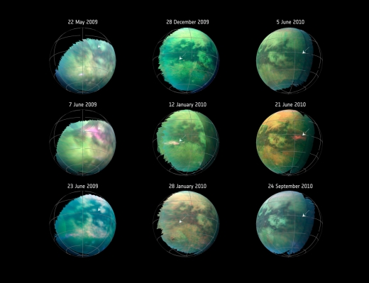
Image: This compilation of images from nine Cassini flybys of Titan in 2009 and 2010 captures three instances when clear bright spots suddenly appeared in images taken by the spacecraft’s Visual and Infrared Mapping Spectrometer. The brightenings were visible only for a short period of time — between 11 hours to five Earth weeks — and cannot be seen in previous or subsequent images. Credit: NASA/JPL-Caltech/University of Arizona/University Paris Diderot/IPGP.
In a paper just published in Nature Geoscience, the researchers likewise discount the possibility that Cassini had detected surface features, areas of frozen methane or lava flows of ice. The problem here is that the bright features in the infrared were visible for relatively short periods — 11 hours to 5 weeks — while surface spots should have remained visible for longer. Nor do they bear the chemical signature expected from such formations at the surface.
Image: This animation — based on images captured by the Visual and Infrared Mapping Spectrometer on NASA’s Cassini mission during several Titan flybys in 2009 and 2010 — shows clear bright spots appearing close to the equator around the equinox that have been interpreted as evidence of dust storms. Credit: NASA/JPL-Caltech/University of Arizona/University Paris Diderot/IPGP.
Rodriguez and team used computer modeling to show that the brightened features were atmospheric but extremely low, forming what is in all likelihood a thin layer of solid organic particles. Such particles form because of the interaction between methane and sunlight. Because the bright features occurred over known dune fields at Titan’s equator, Rodriguez believes that they are clouds of dust kicked up by wind hitting the dunes.
“We believe that the Huygens Probe, which landed on the surface of Titan in January 2005, raised a small amount of organic dust upon arrival due to its powerful aerodynamic wake,” says Rodriguez. “But what we spotted here with Cassini is at a much larger scale. The near-surface wind speeds required to raise such an amount of dust as we see in these dust storms would have to be very strong — about five times as strong as the average wind speeds estimated by the Huygens measurements near the surface and with climate models.”
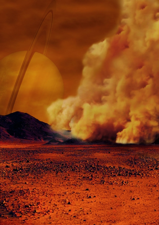
Image: Artist’s concept of a dust storm on Titan. Researchers believe that huge amounts of dust can be raised on Titan, Saturn’s largest moon, by strong wind gusts that arise in powerful methane storms. Such methane storms, previously observed in images from the international Cassini spacecraft, can form above dune fields that cover the equatorial regions of this moon especially around the equinox, the time of the year when the Sun crosses the equator. Credit: NASA/ESA/IPGP/Labex UnivEarthS/University Paris Diderot.
In reaching this conclusion, the researchers analyzed Cassini spectral data and deployed atmospheric models and simulations to show that micrometer-sized solid organic particles from the dunes below were responsible, an indication of dust in the atmosphere that far exceeds what Huygens found at the surface. The winds associated with the phenomenon would be unusually strong, but could be explained by downbursts in the equinoctial methane storms.
If dust storms can be created by such winds, then Titan’s equatorial regions are still active, with the dunes undergoing constant change. We have a world that is active not only in its hydrocarbon cycle and its geology, but also in what we can call its ‘dust cycle.’ The only moon in the Solar System with a dense atmosphere and surface liquid offers yet another analogy with Earth, a similarity that highlights the complexity of this frigid, hydrocarbon-rich world.
The paper is Rodriguez et al., “Observational evidence for active dust storms on Titan at equinox,” Nature Geoscience 24 September 2018 (abstract).

‘Oumuamua’s Origin: A Work in Progress
The much discussed interstellar wanderer called ‘Oumuamua made but a brief pass through our Solar System, and was only discovered on the way out in October of last year. Since then, the question of where the intriguing interloper comes from has been the object of considerable study. This is, after all, the first object known to be from another star observed in our system. Today we learn that a team of astronomers led by Coryn Bailer-Jones (Max Planck Institute for Astronomy) has been able to put Gaia data and other resources to work on the problem.
The result: Four candidate stars identified as possible home systems for ‘Oumuamua. None of these identifications is remotely conclusive, as the researchers make clear. The significance of the work is in the process, which will be expanded as still more data become available from the Gaia mission. So in a way this is a preview of a much larger search to come.
What we are dealing with is the reconstruction of ‘Oumuamua’s motion before it encountered our Solar System, and here the backtracking become tangled with the object’s trajectory once we actually observed it. Its passage through the system as well as stars it encountered before it reached us all factor into determining its origin.
What the Bailer-Jones teams brings to the table is something missing in earlier attempts to solve the riddle of ‘Oumuamua’s home. We learned in June of 2018 that ‘Oumuamua’s orbit was not solely the result of gravitational influences, but that a tiny additional acceleration had been added when the object was close to the Sun. That brought comets into the discussion: Was ‘Oumuamua laden with ice that, sufficiently heated, produced gases that accelerated it?
The problem with that idea was that no such outgassing was visible on images of the object, the way it would be with comets imaged close to the Sun. Whatever the source of the exceedingly weak acceleration, though, it had to be factored into any attempt to extrapolate the object’s previous trajectory. Bailer-Jones and team manage to do this, offering a more precise idea of the direction from which the object came.
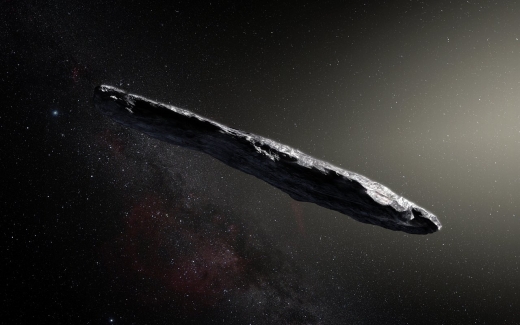
Image: This artist’s impression shows the first interstellar asteroid: `Oumuamua. This unique object was discovered on 19 October 2017 by the Pan-STARRS 1 telescope in Hawai`i. Subsequent observations from ESO’s Very Large Telescope in Chile and other observatories around the world show that it was travelling through space for millions of years before its chance encounter with our star system. `Oumuamua seems to be a dark red object, either elongated, as in this image, or else shaped like a pancake. Credit: ESO/M. Kornmesser.
At the heart of this work are the abundant data being gathered by the Gaia mission, whose Data Release 2 (DR2) includes position, on-sky motion and parallax information on 1.3 billion stars. As this MPIA news release explains, we also have radial velocity data — motion directly away from or towards the Sun — of 7 million of these Gaia stars. The researchers then added in Simbad data on an additional 220,000 stars to retrieve further radial velocity information.
To say this gets complicated is a serious understatement. 4500 stars turn up as potential homes for ‘Oumuamua, assuming both the object and the stars under consideration all moved along straight lines and at constant speeds. Then the researchers had to take into consideration the gravitational influence of all the matter in the galaxy. The likelihood is that ‘Oumuamua was ejected from a planetary system during the era of planet formation, and that it would have been sent on its journey by gravitational interactions with giant planets in the infant system.
Calculating its trajectory, then, could lead us back to ‘Oumuamua’s home star, or at least to a place close to it. Another assumption is that the relative speed of ‘Oumuamua and its parent star is comparatively slow, because objects are not typically ejected from planetary systems at high speed. Given all this, Bailer-Jones and team come down from 4500 candidates to four that they consider the best possibilities. None of these stars is currently known to have planets at all, much less giant planets, but none has been seriously examined for planets to this point.
Let’s pause on this issue, because it’s an interesting one. Digging around in the paper, I learned that unstable gas giants would be more likely to eject planetesimals than systems with stable giant planets, a consequence of the eccentric orbits of multiple gas giants during an early phase of system instability. It also turns out that there are ways to achieve higher ejection velocities. Does ‘Oumuamua come from a binary star? Let me quote from the paper on this:
Higher ejection velocities can occur for planetesimals scattered in a binary star system. To demonstrate this, we performed a simple dynamical experiment on a system comprising a 0.1 M? star in a 10 au circular orbit about a 1.0 M? star. (This is just an illustration; a full parameter study is beyond the scope of this work.) Planetesimals were randomly placed between 3 au and 20 au from the primary, enveloping the orbit of the secondary… Once again most (80%) of the ejections occur at velocities lower than 10 km s?1, but a small fraction is ejected at higher velocities in the range of those we observe (and even exceeding 100 km s?1).
So keep this in mind in evaluating the candidate stars. One of these is the M-dwarf HIP 3757, which can serve as an example of how much remains to be done before we can claim to know ‘Oumuamua’s origin. Approximately 77 light years from Earth, the star as considered by these methods would have been within 1.96 light years of ‘Oumuamua about 1 million years ago. This is close enough to make the star a candidate given how much play there is in the numbers.
But the authors are reluctant to claim HIP 3757 as ‘Oumuamua’s home star because the relative speed between the object and the star is about 25 kilometers per second, making ejection by a giant planet in the home system less likely. More plausible on these grounds is HD 292249, which would have been within a slightly larger distance some 3.8 million years ago. Here we get a relative speed of 10 kilometers per second. Two other stars also fit the bill, one with an encounter 1.1 million years ago, the other at its closest 6.3 million years ago. Both are in the DR2 dataset and have been catalogued by previous surveys, but little is known about them.
Now note another point: None of the candidate stars in the paper are known to have giant planets, but higher speed ejections can still be managed in a binary star system, or for that matter in a system undergoing a close pass by another star. None of the candidates is known to be a binary. Thus the very mechanism of ejection remains unknown, and the authors are quick to add that they are working at this point with no more than a small percentage of the stars that could have been ‘Oumuamua’s home system.
Given that the 7 million stars in Gaia DR2 with 6D phase space information is just a small fraction of all stars for which we can eventually reconstruct orbits, it is a priori unlikely that our current search would find ‘Oumuamua’s home star system.
Yes, and bear in mind too that ‘Oumuamua is expected to pass within 1 parsec of about 20 stars and brown dwarfs every million years. Given all of this, the paper serves as a valuable tightening of our methods in light of the latest data we have about ‘Oumuamua, and points the way toward future work. The third Gaia data release is to occur in 2021, offering a sample of stars with radial velocity data ten times larger than DR2 [see the comments for a correction on this]. No one is claiming that ‘Oumuamua’s home star has been identified, but the process for making this identification is advancing, an effort that will doubtless pay off as we begin to catalog future interstellar objects making their way into our system.
The paper is Bailer-Jones et al., “Plausible home stars of the interstellar object ‘Oumuamua found in Gaia DR2,” accepted for publication in The Astrophysical Journal (preprint).
Hayabusa2: Successful Rover Deployment at Asteroid Ryugu
That small spacecraft can become game-changers, our topic last Friday, is nowhere more evident than in the success of Rover 1A and 1B, diminutive robot explorers that separated from the Hayabusa2 spacecraft at 0406 UTC on September 21 and landed soon after. Their target, the asteroid Ryugu, will be the site of detailed investigation not only by these two rovers, but also by two other landers, the German-built Mobile Asteroid Surface Scout (MASCOT) and Rover 2, the first of which is to begin operations early in October. Congratulations to JAXA, Japan’s space agency, for these early successes delivered by its Hayabusa2 mission.
Surface operations will be interesting indeed. Both rovers were released at an altitude of 55 meters above the surface, their successful deployment marking an advance over the original Hayabusa mission, which was unable to land its rover on the asteroid Itokawa in 2005. Assuming all goes well, the mission should gather three different samples of surface material for return to Earth in 2020. The third sample collection is to take advantage of Hayabusa2’s Small Carry-on Impactor (SCI), which will create a crater to retrieve subsurface material.
Why Ryugu? The object is a carbonaceous asteroid that has likely changed little since the Solar System’s early days, rich in organic material and offering us insight into the kind of objects that would have struck the Earth in the era when life’s raw materials, along with water, could have been delivered. It has also proven, as the JAXA team knew it would, a difficult landing site, with an uneven distribution of mass that produces variations in the gravitational pull over the surface.
On that score, it’s interesting to note that the Hayabusa2 controllers are sharing data with NASA’s OSIRIS-REx mission to asteroid Bennu. Likewise a sample return effort, OSIRIS-REx will face the same gravitational issues inherent in such small, irregular objects, which can be ameliorated by producing maps of each asteroid’s gravity. The three-dimensional models produced for the Dawn spacecraft at Ceres are the kind of software tools that will help both mission teams understand their targets better and ensure successful operations on the surface.
But back to Rover 1A and 1B, which have landed successfully and are both taking photographs and sending data, the first time we have landed and moved a probe autonomously on an asteroid surface. Although the first image was blurred because of the rover’s spin, it did display the receding Hayabusa spacecraft and the bright swath of the asteroid just below. Here’s JAXA’s mission tweet of that first image.
This is a picture from MINERVA-II1. The color photo was captured by Rover-1A on September 21 around 13:08 JST, immediately after separation from the spacecraft. Hayabusa2 is top and Ryugu's surface is below. The image is blurred because the rover is spinning. #asteroidlanding pic.twitter.com/CeeI5ZjgmM
— HAYABUSA2@JAXA (@haya2e_jaxa) September 22, 2018
Says Tetsuo Yoshimitsu, who leads the MINERVA-II1 rover team:
Although I was disappointed with the blurred image that first came from the rover, it was good to be able to capture this shot as it was recorded by the rover as the Hayabusa2 spacecraft is shown. Moreover, with the image taken during the hop on the asteroid surface, I was able to confirm the effectiveness of this movement mechanism on the small celestial body and see the result of many years of research.
The ‘hop’ Yoshimitsu refers to is a reference to the means of locomotion the rovers will use on the surface. Remember that these vehicles are no more than 18 centimeters wide and 7 centimeters high, weighing on the order of 1 kilogram. In Ryugu’s light gravity, the rovers will make small jumps across the surface, a motion carefully constrained so as not to reach the object’s escape velocity. Below is the first Rover-1A image taken during a hop.
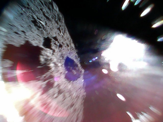
Image: Captured by Rover-1A on September 22 at around 11:44 JST. Color image captured while moving (during a hop) on the surface of Ryugu. The left-half of the image is the asteroid surface. The bright white region is due to sunlight. Credit: JAXA.
And have a look at an image taken during landing operations before Rover-1B reached the surface. Here the asteroid terrain is clearly defined.
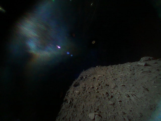
Image: Captured by Rover-1B on September 21 at around 13:07 JST. This color image was taken immediately after separation from the spacecraft. The surface of Ryugu is in the lower right. The coloured blur in the top left is due to the reflection of sunlight when the image was taken. Credit: JAXA.
Yuichi Tsuda is Hayabusa2 project manager:
I cannot find words to express how happy I am that we were able to realize mobile exploration on the surface of an asteroid. I am proud that Hayabusa2 was able to contribute to the creation of this technology for a new method of space exploration by surface movement on small bodies.
I would say Tsuda’s pride in his team and his hardware is more than justified. As we go forward with surface operations, let me commend Elizabeth Tasker’s fine work in spreading JAXA news in English. Even as JAXA offers live updates from Hayabusa2 in English and the official Hayabusa2 site offers its own coverage, Tasker, a British astrophysicist working at JAXA, has provided useful mission backgrounders like this one, as well as running the English-language Hayabusa2 Twitter account @haya2e_jaxa, and keeping up with her own Twitter account @girlandkat. There will be no shortage of Ryugu news in days ahead.
MarCO: Taking CubeSat Technologies Interplanetary
The image below intrigues me. It’s the first image of the Earth and the Moon together taken from a CubeSat, one of a pair of such tiny spacecraft NASA has despatched to Mars as part of a mission called MarCO (Mars Cube One), which will work in conjunction with the InSight lander. Taken on May 9, the photo was part of the process of testing the CubeSat’s high-gain antenna. But to me it’s a reminder of how far miniaturized technologies continue to advance.
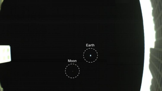
Image: The first image captured by one of NASA’s Mars Cube One (MarCO) CubeSats. The image, which shows both the CubeSat’s unfolded high-gain antenna at right and the Earth and its moon in the center, was acquired by MarCO-B on May 9. Credit: NASA/JPL-Caltech.
As of this morning, we are 66 days away from InSight’s landing on Mars, at a distance of 65 million kilometers from Earth and 16 million kilometers to Mars. I don’t usually focus on Mars and lunar missions because this site’s specialty is deep space, which for our purposes means Jupiter and beyond, and of course the overall theme here is interstellar. But experimental technologies that bring us greater performance from very small payloads are certainly relevant.
Anything we can do to shrink payload size pays off as we look at ever more distant targets, and the cruise velocities and propellant needed to reach them. And CubeSats are a way of exploring small payloads. The standard 10×10×11 cm basic CubeSat is a ‘one unit’ (1U) CubeSat, but larger platforms of 6U and 12U allow more complex missions. With fixed satellite body dimensions, the CubeSat format creates a highly modular and integrated system.
What we have with the two MarCO spacecraft is the application of what had been a low-Earth orbit satellite technology to a planetary mission, with a useful goal. Trailing InSight by thousands of kilometers, they’ve already demonstrated their ability to operate in the interplanetary environment. At Mars, the intention is for them to relay data on InSight’s landing, a job consigned to Mars orbiters, but one this mission may show CubeSats are able to perform.
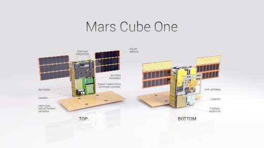
Image: Illustration of one of the twin MarCO spacecraft with some key components labeled. Front cover is left out to show some internal components. Antennas and solar arrays are in deployed configuration. Credit: NASA/JPL-Caltech.
Each of the MarCOs has its own high-gain antenna and the necessary radio equipment for data relay, with propulsion systems that have already made two steering maneuvers enroute. No one would claim the diminutive space travelers are as complex as conventional interplanetary craft, but I can see two goals here, the first of which leverages the ‘traditional’ CubeSat role of acting as low-cost entry-level ways to reach orbit.
“Our hope is that MarCO could help democratize deep space,” said Jakob Van Zyl, director of the Solar System Exploration Directorate at NASA’s Jet Propulsion Laboratory in Pasadena, California. “The technology is cheap enough that you could envision countries entering space that weren’t players in the past. Even universities could do this.”
Fair enough, as we’ve learned how satellites can be ‘piggybacked’ to open up access to space, lowering launch costs even as the cost of the CubeSats offers opportunities for inexpensive missions. Moreover, the fact that CubeSats can be built with standardized parts and systems, with key components provided by commercial partners, underscores their efficiency.
But let’s move beyond today’s current CubeSat. If we can build these craft strong enough to handle relay operations from Mars, we can contemplate future CubeSats capable of a wider range of science return and consider propulsion technologies like solar sails for ‘swarm’ missions to targets beyond Mars. Of particular interest is coupling CubeSats with solar sails for propulsion. Remember, for example, The Planetary Society’s LightSail-1, launched in 2015, which demonstrated sail deployment despite a series of major software glitches.
LightSail-2 is designed to demonstrate controlled solar sailing in the CubeSat format, with a sail of 32 square meters. A key goal of this mission is to raise the orbit apogee after sail deployment at 720 kilometers. I should also mention LightSail-3, which could take this technology out to the L1 Lagrangian point, where it would remain to monitor geomagnetic activity on the Sun.
NASA’s own future plans for CubeSat work take in BioSentinel, which would take living yeast (S. cerevisiae) into space to study DNA lesions caused by energetic particles, with operations expected to last 18 months at distances well beyond low Earth orbit. The NEA (Near-Earth Asteroid) Scout mission would take a CubeSat/sail to a small asteroid, exploring its rotational properties, spectral class, regional morphology and regolith, while Lunar Flashlight would achieve lunar orbit to study ice deposits on the Moon for the use of future explorers.
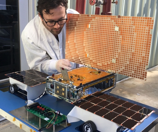
Image: Engineer Joel Steinkraus uses sunlight to test the solar arrays on one of the Mars Cube One (MarCO) spacecraft. Credit: NASA/JPL-Caltech.
I might likewise mention such European Space Agency efforts as GOMX-3, a CubeSat mission exploring the telecommunications capabilities of such craft. GOMX-3 was deployed from the International Space Station in October of 2015 and operated for a year before re-entering the atmosphere.
The list of upcoming missions under ESA’s In-Orbit Demonstration is extensive (you can see it here), and it’s noteworthy that the agency inserts at the top of its list of potential applications the fact that CubeSats can serve “As a driver for drastic miniaturisation of systems, ‘systems-on-chips’, and totally new approach to packaging and integration, multi-functional structures, embedded propulsion.”
So we can keep an eye on the MarCOs as a harbinger of CubeSat operations to come. All three of the future NASA CubeSat missions I’ve mentioned are designed to be launched as secondary payloads on a future Space Launch System (SLS) mission. But however we get such missions into space, they point toward further exploration of small payloads, a parameter space Breakthrough Starshot is pushing to the max in its plans for a centimeter-sized, gram-scale payload to be driven by laser propulsion at 20 percent of lightspeed to another star.
Ceres: Of Ice and Volcanoes
We’ve only orbited one object in the Solar System known to exhibit cryovolcanism, but Ceres has a lot to teach us about the subject. Unlike the lava-spewing volcanoes of Earth, an ice volcano can erupt with ammonia, water or methane in liquid or vapor form. What appear to be cryovolcanoes can be found not only on Ceres but Titan, and the phenomenon appears likely on Pluto and Charon. Neptune’s moon Triton is a special case, with rugged volcanic terrain in evidence, as opposed to much smoother surfaces without obvious volcanoes elsewhere.
Activity like this can be a good deal less dramatic than what we see on Earth, or spectacularly on Io. The eruption of an ice volcano involves rocks, ice and volatiles more or less oozing up out of the volcano to freeze on the surface, a process thought to be widespread on Ceres. But what happens to cryovolcanoes as they age? Ahuna Mons, an almost five-kilometer tall mountain that is no more than 200 million years old, raises the question. Why is it so tall, and why, assuming other cryovolcanic activity on this surface, are there no other mountains this imposing?
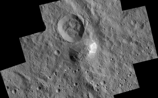
Image: Ceres’ unusual mountain Ahuna Mons is seen in this mosaic of images from NASA’s Dawn spacecraft. On its steepest side, this mountain is about 5 kilometers high. Its average overall height is 4 kilometers. The diameter of the mountain is about 20 kilometers. Dawn took these images from its low-altitude mapping orbit in December 2015. Credit: NASA/JPL/Dawn mission.
Tackling the question of cryovolcano evolution is Michael Sori (University of Arizona), working with colleagues at UA and elsewhere to advance a theory they call ‘viscous relaxation.’ The idea here is that the rock and ice making up Ceres can flow in much the way that glaciers flow on Earth, with the ice/rock balance affecting the flow rate. Also a key factor: The temperature, which on Ceres never warms higher than -35 degrees Celsius. A cryovolcano at the poles, in other words, would ‘relax’ at a much slower rate than a warmer mountain at the equator.
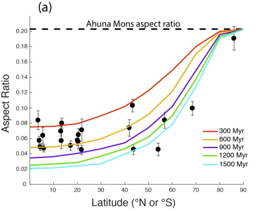
Image: Each curve represents a cryovolcano of a different age and shows that mountains at low latitudes close to the equator flatten out at younger ages than mountains located at high latitudes at the poles, where they will maintain their height and width for eons. Credit: Michael Sori.
The youthful Ahuna Mons would have been active in the geologically recent past. In a paper published in 2017, Sori’s team used numerical models to predict the flow velocity of the cryovolcano, which they derive as 10-500 meters per million years given the variables of ice content, rheology (the deformation and flow of matter), grain size, and temperature. Flows at the slow end of this range can relax a cryovolcanic structure over 108 to 109 years, a rate sufficient to allow Ahuna Mons to remain identifiable today.
Older cryovolcanoes, having gone lengthier periods of relaxation, become shorter, wider and more rounded with the passage of time. The trick is to identify ancient cryovolcanic structures on today’s surface. In a paper just released in Nature Astronomy, the scientists used their computer simulations as the context in which to scan Dawn data on Ceres’ topography.
22 surface features matched the simulation’s predictions, including Yamor Mons, an old polar mountain five times wider than it is tall. Mountains elsewhere on the surface of the dwarf planet have lower aspect ratios; that is, they are much wider than they are tall. Sori’s team was able to use the simulation/data match to estimate the age of many volcanoes and their volume.
Viscous relaxation as modeled here allows the researchers to derive the rate at which cryovolcanoes form, which turns out to be one every 50 million years. Ceres shows signs of cryovolcanism throughout its history, making the process an important factor in its geological evolution, though less so than the kind of volcanism found on terrestrial planets. Depending on latitude, modeled volcanoes begin tall and steep, but grow short and wide over time.
This passage from the 2017 paper summarizes the process of cryovolcano evolution. Note the acronym FEM, standing for ‘finite element method,’ a reference to software code originally developed for the study of the movement of ice on Earth and used in these simulations
Viscous flow of topography is a modification mechanism that can describe the presence of a single, young, prominent cryovolcano (Ahuna Mons). Flow velocities are fast enough to heavily modify structures on timescales of tens to hundreds of million years, shallowing their topographic relief and providing an explanation for why Dawn observations have not yet identified a plethora of cryovolcanoes. Flow velocities are not so fast that the observed near-pristine state of Ahuna Mons becomes problematic. Domes must be more compositionally ice rich than the average Cerean crust to flow, which is a reasonable property for a cryovolcanic construct. Our hypothesis works with any volumetric fraction of ice > ~40%, but we favor the lower end of this range because past studies do not favor a pure-ice composition for Ahuna Mons. Cerean cryovolcanism involving cryomagma that is approximately half water by volume fits both Dawn observations and our FEM models.
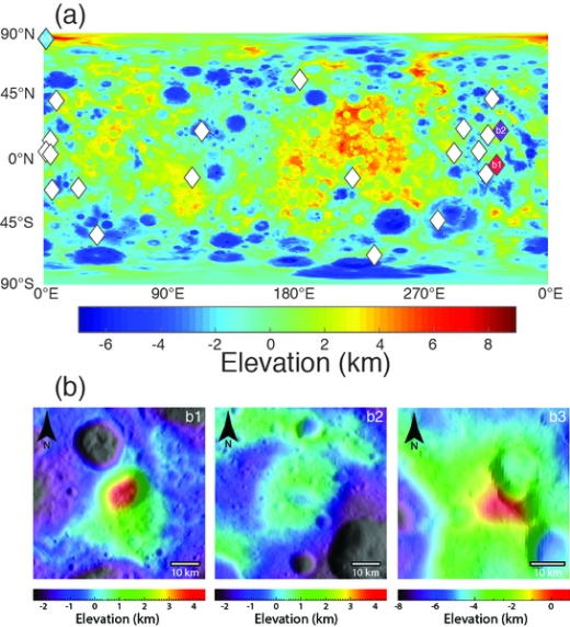
Image: A topographic map of Ceres (top), with the dark red representing the highest elevations and dark blue being the lowest. The topography of Ahuna Mons is shown on the bottom left, and Yamor Mons is shown on the bottom right. The bottom center image shows the topography of an ancient cryovolocano located north of Ceres’s equator. Credit: Michael Sori.
Cryovolcanoes aren’t dramatic. We substitute an ooze of cryomagma, a mixture of rock, salty ice and volatiles, for explosive eruptions. Freezing on the surface, the cryomagma eventually rises into peaks like Ahuna Mons before the inevitable relaxation as geological ages pass. How and why the cryovolcanic activity occurs just where it does is a question for future research, and one that may be illuminated by studies of the ice volcanoes elsewhere in the Solar System.
The paper is Sori et al., “Cryovolcanic rates on Ceres revealed by topography,” Nature Astronomy 17 September 2018 (abstract). The earlier paper is Sori et al., “The vanishing cryovolcanoes of Ceres,” Geophysical Research Letters Vol. 44, Issue 3 (16 February 2017) 1243-1250 (abstract).
Looking Back at Titan
There are two senses in which we are ‘looking back’ at Titan in today’s post. On the one hand, the New Horizons spacecraft has already taken sensors well beyond Pluto in preparation for the encounter with MU69. From its perspective, anything in the Solar System inside the Kuiper Belt is well behind. What with our Pioneers, Voyagers and now New Horizons, the human perspective has widened that far.
But we’re also looking back in terms of time when we revisit the Cassini mission and what it had to tell us about Saturn’s moons. Below is the final view the spacecraft had of Titan’s lakes and seas, a view of the north polar terrain showing the abundance of liquid methane and ethane. The view was acquired on September 11, 2017, a mere four days before Cassini was sent to its fiery end in Saturn’s atmosphere as a way of avoiding any potential future contamination.
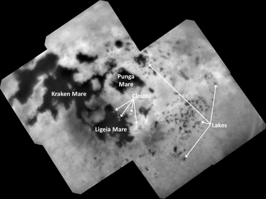
Image: This view of Titan’s northern polar landscape was obtained at a distance of approximately 140,000 kilometers (87,000 miles) from Titan. Image scale is about 800 meters (0.5 miles) per pixel. The image is an orthographic projection centered on 67.19 degrees north latitude, 212.67 degrees west longitude. An orthographic view is most like the view seen by a distant observer looking through a telescope. Credit: NASA/JPL-Caltech/Space Science Institute.
Just above the center of this mosaic is Punga Mare, 390 kilometers (240 miles) across, with Ligeia Mare (500 kilometers, or 300 miles wide) below center. The large body of methane/ethane at left is Kraken Mare, some 1200 kilometers across (730 miles). Note the scattering of small lakes around the seas, especially at the right side of the mosaic.
Also interesting is the small amount of cloud cover, though a few do appear just below center in the image, as well as several above Ligeia Mare. We would expect clouds, since Titan’s methane cycle involves rainfall, surface runoff, collected methane in large bodies like these, and evaporation, much like Earth’s water cycle. And in fact, cloud activity was found during southern summer over the south pole. But here we’re in northern spring and summer, with few clouds.
“We expected more symmetry between the southern and northern summer,” said Elizabeth (“Zibi”) Turtle of the Johns Hopkins Applied Physics Lab and the Cassini Imaging Science Subsystem (ISS) team that captured the image. “In fact, atmospheric models predicted summer clouds over the northern latitudes several years ago. So, the fact that they still hadn’t appeared before the end of the mission is telling us something interesting about Titan’s methane cycle and weather.”
Remember that among the many things Cassini found on Titan are two different kinds of methane/ethane-filled depressions that create the features we see in this mosaic. Some are responsible for the collection of the large seas, which are not only hundreds of kilometers across but evidently several hundred meters deep, all fed by branching channels like rivers on Earth. The much smaller lakes show terrain with steep walls and rounded edges. They do not appear to be associated with incoming channels, meaning they are filled by rainfall or by upwelling from below, and it’s known that some of them fill and dry out during Titan’s seasonal cycle.
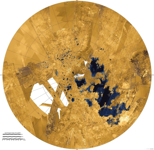
Image: An earlier, colorized mosaic from NASA’s Cassini mission shows Titan’s northern land of lakes and seas. Here the data were obtained from 2004 to 2013. In this projection, the north pole is at the center. The view extends down to 50 degrees north latitude. In this color scheme, liquids appear blue and black depending on the way the radar bounced off the surface. Land areas appear yellow to white. Credit: NASA/JPL-Caltech/Space Science Institute.
In a 2015 study, Thomas Cornet (European Space Agency) and colleagues went to work on Titan’s lakes, noting that they are reminiscent of ‘karstic’ landforms on Earth. On our planet, these result from erosion due to groundwater and rainfall affecting dissolvable rock such as limestone and gypsum, creating both caves and sinkholes or, in desert climates, salt pans.
Cornet’s team worked out how long it would take to create features like this on Titan, assuming a surface covered in organic material, with the main dissolving agent being liquid hydrocarbons operating in a climate based on current models. The result: 50 million years to create a 100-meter (330 ft) depression in the polar regions. Says Cornet:
“We compared the erosion rates of organics in liquid hydrocarbons on Titan with those of carbonate and evaporite minerals in liquid water on Earth. We found that the dissolution process occurs on Titan some 30 times slower than on Earth due to the longer length of Titan’s year and the fact it only rains during Titan summer. Nonetheless, we believe that dissolution is a major cause of landscape evolution on Titan and could be the origin of its lakes.”
Thus we find a process of erosion dependent on rock chemistry, rainfall rate and surface temperature that has similarities with what we see on Earth on what Cornet calls a “relatively youthful billion-year-old surface,” a comparatively slow surface transformation that is even slower at lower latitudes, where the rainfall is less frequent. For more on this, see New Insights into Titan.
The Cornet paper on Titan’s surface features is “Dissolution on Titan and on Earth: Towards the age of Titan’s karstic landscapes,” Journal of Geophysical Research – Planets 25 April 2015 (full text).

Follow with RSS or E-Mail
